

Introduction: The Physics of Rhythm in Our World
Every morning, your alarm clock vibrates to wake you up. As you walk, your arms swing naturally at your sides. The suspension system in your car smooths out bumps in the road. Your smartphone’s accelerometer detects motion through tiny oscillating components. Even your heartbeat follows a rhythmic pattern that doctors monitor for your health.
These seemingly different phenomena all share a fundamental physics principle: oscillation. From the microscopic vibrations of atoms in a crystal lattice to the massive oscillations of skyscrapers during earthquakes, oscillatory motion governs much of the physical world around us. Understanding oscillations isn’t just about passing your AP Physics C exam-it’s about comprehending one of nature’s most universal patterns.
In this comprehensive guide, you’ll master Unit 7 of AP Physics C: Mechanics, diving deep into the mathematical beauty and practical applications of oscillatory systems. Whether you’re struggling with the conceptual foundations or looking to perfect your problem-solving techniques for the most challenging free-response questions, this guide will transform your understanding of oscillations from confusing equations into intuitive physical insight.
Learning Objectives: Your Roadmap to Oscillation Mastery
By the end of this unit, you should confidently demonstrate these College Board-aligned competencies:
Conceptual Understanding:
- Explain the conditions necessary for simple harmonic motion and identify when systems exhibit this behavior
- Distinguish between different types of oscillating systems and their unique characteristics
- Analyze the relationship between restoring forces and harmonic motion
- Connect energy transformations in oscillating systems to conservation principles
Mathematical Proficiency:
- Derive and apply the fundamental equations governing simple harmonic motion
- Solve complex problems involving springs, pendulums, and combined oscillating systems
- Analyze oscillatory motion using both algebraic and graphical approaches
- Calculate periods, frequencies, amplitudes, and phase constants for various scenarios
Laboratory Skills:
- Design experiments to investigate oscillatory systems and measure their properties
- Analyze data from oscillation experiments and determine system parameters
- Evaluate uncertainties in oscillation measurements and their propagation through calculations
- Connect theoretical predictions with experimental observations
Problem-Solving Expertise:
- Apply multiple approaches to solve oscillation problems (energy methods, force analysis, differential equations)
- Recognize and correct common misconceptions about oscillatory motion
- Tackle multi-step problems involving combinations of translational and rotational oscillations
- Prepare effectively for AP exam question formats specific to this unit
1: The Foundations of Simple Harmonic Motion
Understanding the Heartbeat of Physics
Simple harmonic motion represents one of the most elegant examples of mathematical physics in action. At its core, simple harmonic motion occurs whenever a system experiences a restoring force that’s directly proportional to its displacement from equilibrium. This seemingly simple relationship gives rise to incredibly rich and complex behaviors that appear throughout the natural world.
Think about a mass attached to a spring lying on a frictionless surface. When you pull the mass away from its equilibrium position, the spring exerts a force trying to restore the system to balance. The farther you stretch the spring, the stronger this restoring force becomes. This linear relationship between displacement and restoring force is the hallmark of simple harmonic motion.
Real-World Physics: The same principle governs the oscillation of atoms in crystalline solids. When atoms are displaced slightly from their equilibrium positions, electromagnetic forces create restoring forces proportional to displacement. This atomic-level simple harmonic motion determines many material properties, including thermal expansion, specific heat, and even electrical conductivity in some materials.
The Mathematical Heart: Hooke’s Law and Beyond
The foundation of simple harmonic motion rests on Hooke’s Law, but understanding its deeper implications requires careful analysis. When we write:
[EQUATION: F = -kx, where F is the restoring force, k is the spring constant, and x is displacement from equilibrium]
The negative sign carries profound physical meaning. It indicates that the force always opposes displacement, always trying to restore equilibrium. This creates the oscillatory behavior we observe.
Applying Newton’s second law to this restoring force gives us the fundamental differential equation of simple harmonic motion:
[EQUATION: ma = -kx, which becomes m(d²x/dt²) = -kx, or d²x/dt² + (k/m)x = 0]
This differential equation has a well-known solution that describes all simple harmonic motion:
[EQUATION: x(t) = A cos(ωt + φ), where A is amplitude, ω = √(k/m) is angular frequency, and φ is the phase constant]
Each parameter in this equation carries physical significance. The amplitude A represents the maximum displacement from equilibrium-essentially how “big” the oscillation is. The angular frequency ω determines how rapidly the system oscillates, directly related to the system’s physical properties. The phase constant φ tells us about the initial conditions: where the oscillation starts and in which direction it’s initially moving.
Energy in Oscillating Systems: A Dance Between Kinetic and Potential
One of the most beautiful aspects of simple harmonic motion is how energy continuously transforms between kinetic and potential forms while the total mechanical energy remains constant (in the absence of friction).
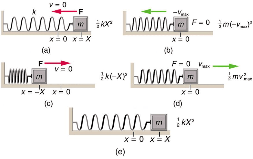
At the moment of maximum displacement (when x = ±A), the system momentarily stops before reversing direction. All energy exists as elastic potential energy:
[EQUATION: PE_max = ½kA², representing maximum potential energy storage]
As the system passes through equilibrium (x = 0), all energy has transformed into kinetic energy:
[EQUATION: KE_max = ½mv_max², where v_max = ωA]
At any intermediate position, energy exists in both forms:
[EQUATION: E_total = ½kx² + ½mv² = ½kA² = constant]
This energy perspective often provides the most elegant approach to solving oscillation problems, especially when dealing with complex systems where force analysis becomes cumbersome.
Physics Check: Can you explain why the total energy of a simple harmonic oscillator is proportional to the square of its amplitude? This relationship has important implications for wave intensity and sound loudness in real-world applications.
2: The Mathematics of Oscillation
Period and Frequency: Timing the Universe
The period T of simple harmonic motion represents the time required for one complete oscillation cycle. For a mass-spring system, this period depends only on the system’s inherent properties:
[EQUATION: T = 2π√(m/k), showing period increases with mass and decreases with spring stiffness]
This relationship reveals something profound about oscillatory systems: the period is independent of amplitude. Whether you stretch a spring by 1 centimeter or 10 centimeters, it will complete each oscillation cycle in exactly the same time. This principle, known as isochronism, makes pendulum clocks possible and governs the behavior of many natural oscillators.
The frequency f, representing oscillations per unit time, is simply the reciprocal of period:
[EQUATION: f = 1/T = (1/2π)√(k/m) Hz]
Angular frequency ω provides a convenient alternative, especially when dealing with circular motion analogies:
[EQUATION: ω = 2πf = √(k/m) rad/s]
Phase Analysis: Describing Motion at Any Instant
The complete description of simple harmonic motion requires three functions: position, velocity, and acceleration. Starting with the general position function:
[EQUATION: x(t) = A cos(ωt + φ)]
We can derive velocity by taking the time derivative:
[EQUATION: v(t) = dx/dt = -Aω sin(ωt + φ)]
And acceleration by taking the second derivative:
[EQUATION: a(t) = dv/dt = -Aω² cos(ωt + φ) = -ω²x(t)]
Notice that acceleration is always proportional to displacement but in the opposite direction-this is the defining characteristic of simple harmonic motion.
The phase relationships between these quantities reveal important insights. When displacement is maximum (cos term equals ±1), velocity is zero (sin term equals 0). When displacement is zero (cos term equals 0), velocity is maximum (sin term equals ±1). Acceleration is always proportional to displacement but opposite in direction.
Problem-Solving Strategy: When given initial conditions (position and velocity at t = 0), you can determine both amplitude and phase constant:
- A = √(x₀² + (v₀/ω)²)
- φ = arctan(-v₀/(ωx₀))
Differential Equation Solutions and Physical Intuition
The differential equation for simple harmonic motion reveals why oscillation occurs naturally in many physical systems. Any system that experiences a restoring force proportional to displacement will oscillate harmonically.
[EQUATION: d²x/dt² + ω²x = 0]
This second-order linear differential equation has the general solution:
[EQUATION: x(t) = C₁ cos(ωt) + C₂ sin(ωt)]
Which can be rewritten in the more physically intuitive form:
[EQUATION: x(t) = A cos(ωt + φ)]
The constants A and φ are determined by initial conditions, while ω depends entirely on the system’s physical properties.
Historical Context: The mathematical treatment of oscillatory motion was developed primarily by 18th-century mathematicians including Euler, Lagrange, and d’Alembert. Their work on differential equations was motivated largely by problems in mechanics and astronomy, including the analysis of pendulum motion and planetary orbits.
3: Spring Systems and Elastic Oscillations
Single Springs: The Prototype Oscillator
The mass-spring system serves as the archetypal example of simple harmonic motion because it perfectly embodies the linear restoring force relationship. When we attach a mass m to a spring with spring constant k, we create a system whose behavior we can predict with remarkable precision.
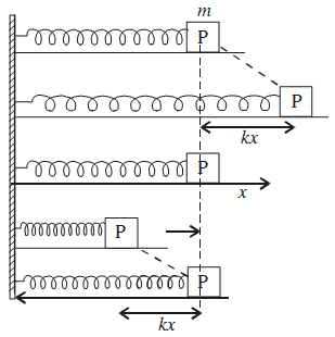
For a horizontal mass-spring system (where gravity doesn’t affect the motion), the analysis is straightforward. The spring provides a restoring force F = -kx, leading to the familiar period formula:
[EQUATION: T = 2π√(m/k)]
However, vertical spring systems require more careful analysis. When we hang a mass from a vertical spring, gravity stretches the spring to a new equilibrium position. At this new equilibrium, the spring force exactly balances the gravitational force:
[EQUATION: kx₀ = mg, where x₀ is the equilibrium stretch]
Remarkably, oscillations about this new equilibrium position follow exactly the same mathematical form as horizontal oscillations. The period remains T = 2π√(m/k), independent of gravitational effects.
Common Error Alert: Students often incorrectly include gravitational effects in vertical spring oscillation problems. Remember that gravity only shifts the equilibrium position; it doesn’t change the oscillatory behavior about that equilibrium.
Springs in Series and Parallel: Building Complex Systems
Real-world oscillating systems often involve multiple springs connected in various configurations. Understanding how to analyze these combinations is crucial for both exam success and practical applications.
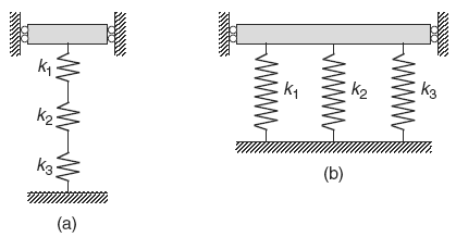
Springs in Series:
When springs are connected end-to-end, they share the same force but experience different extensions. The effective spring constant for springs in series is:
[EQUATION: 1/k_eff = 1/k₁ + 1/k₂ + 1/k₃ + …]
This means springs in series are collectively “softer” than any individual spring—the effective spring constant is always less than the smallest individual spring constant.
Springs in Parallel:
When springs are connected side-by-side, they share the same displacement but provide additive forces. The effective spring constant for springs in parallel is:
[EQUATION: k_eff = k₁ + k₂ + k₃ + …]
Springs in parallel create a “stiffer” system than any individual spring alone.
Real-World Physics: Car suspension systems use both series and parallel spring arrangements. The main springs support the vehicle weight (parallel arrangement for load distribution), while additional springs and dampers in series provide fine-tuning for ride comfort and handling.
Energy Methods in Spring Analysis
Energy conservation provides a powerful alternative to force analysis, especially for complex spring systems. The total mechanical energy of an oscillating spring system remains constant:
[EQUATION: E = ½kA² = ½kx² + ½mv²]
This energy approach proves particularly valuable when analyzing non-uniform motion or when position-dependent forces make direct integration difficult.
For example, when finding the speed of a mass at any position during its oscillation:
[EQUATION: v = ±ω√(A² – x²)]
The ± sign indicates that the mass can be moving in either direction at any given position (except at the turning points where v = 0).
4: Pendulum Motion and Gravitational Oscillations
The Simple Pendulum: Gravity’s Timekeeper
The simple pendulum-a point mass suspended by a massless, inextensible string-represents one of the most historically significant oscillating systems in physics. From Galileo’s observations in the cathedral of Pisa to modern atomic clocks, pendulums have shaped our understanding of time and motion.
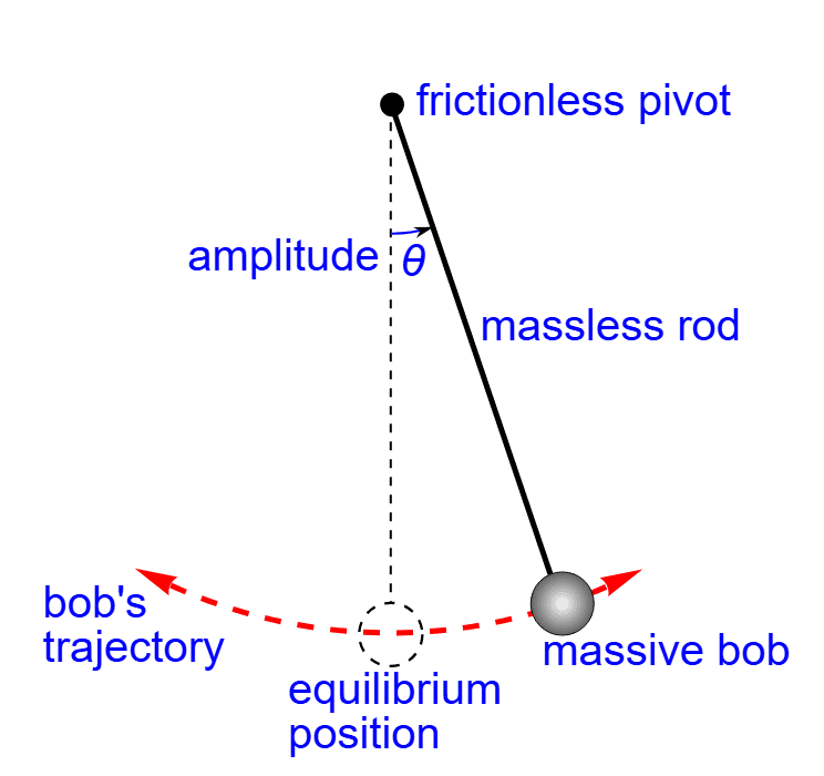
For small angular displacements (typically less than 15°), the restoring torque on a pendulum is proportional to angular displacement:
[EQUATION: τ = -mgL sin(θ) ≈ -mgLθ for small θ]
This leads to simple harmonic motion with period:
[EQUATION: T = 2π√(L/g)]
This remarkable result shows that the period depends only on length and local gravitational acceleration—it’s independent of the pendulum’s mass or amplitude (for small oscillations).
Physics Check: Why does the period of a simple pendulum not depend on the bob’s mass? This counterintuitive result occurs because both the restoring torque and the rotational inertia are proportional to mass, so mass cancels out of the equation of motion.
The Physical Pendulum: Real-World Complexity
Most real pendulums are not point masses but extended objects with distributed mass. These physical pendulums require more sophisticated analysis using rotational dynamics.
For a physical pendulum, the restoring torque about the pivot point is:
[EQUATION: τ = -mgd sin(θ) ≈ -mgdθ for small θ]
where d is the distance from the pivot to the center of mass.
The equation of motion becomes:
[EQUATION: Iα = -mgdθ, where I is the moment of inertia about the pivot]
This yields the period formula for physical pendulums:
[EQUATION: T = 2π√(I/(mgd))]
Problem-Solving Strategy: For physical pendulums, always use the parallel axis theorem to find the moment of inertia about the pivot point:
[EQUATION: I_pivot = I_cm + md²]
Large Amplitude Oscillations: When Simple Approximations Break Down
For large angular displacements, the small angle approximation (sin θ ≈ θ) becomes inaccurate, and pendulum motion is no longer simple harmonic. The period increases with amplitude according to:
[EQUATION: T = T₀[1 + (1/16)θ₀² + (11/3072)θ₀⁴ + …] where T₀ = 2π√(L/g)]
This series expansion shows that for a 30° amplitude, the period increases by about 1.7% compared to small oscillations. While this might seem small, such corrections become crucial in precision timekeeping applications.
Real-World Physics: The world’s most accurate pendulum clocks account for these nonlinear effects, along with temperature variations that change the pendulum length, air pressure changes that affect buoyancy, and even the slight variations in Earth’s gravitational field due to tidal effects from the moon and sun.
5: Energy and Conservation in Oscillatory Systems
The Energy Landscape of Oscillation
Understanding oscillatory systems through energy analysis often provides deeper insight than force-based approaches. In simple harmonic motion, energy constantly transforms between kinetic and potential forms, but the total mechanical energy remains constant.
The potential energy function for a harmonic oscillator creates a parabolic “well”:
[EQUATION: U(x) = ½kx²]
This parabolic potential energy curve explains why small displacements from equilibrium lead to simple harmonic motion. Near the minimum of any smooth potential energy function, the force law becomes approximately linear (Hooke’s law), resulting in harmonic oscillation.
The total energy determines the amplitude of oscillation:
[EQUATION: E = ½kA² = U_max = KE_max]
At the turning points (x = ±A), all energy is potential. At equilibrium (x = 0), all energy is kinetic.
Energy Methods for Complex Systems
Energy conservation provides elegant solutions to problems that would be extremely difficult using force analysis. Consider a mass oscillating on a spring attached to an inclined plane. While the force analysis requires careful vector decomposition, energy methods give immediate results:
[EQUATION: ½kx² + ½mv² + mgx sin(θ) = constant]
where θ is the angle of inclination.
Problem-Solving Strategy: Energy methods work best when:
- You need to find speeds at specific positions
- The system involves conservative forces only
- Force analysis becomes mathematically complex
- You’re dealing with multiple connected oscillators
Damped Oscillations: Energy Loss in Real Systems
Real oscillators always experience some form of energy dissipation—friction, air resistance, internal material losses, or electrical resistance. These effects cause the amplitude to decrease over time while (usually) leaving the frequency nearly unchanged.
For lightly damped systems, the motion can be described by:
[EQUATION: x(t) = Ae^(-γt) cos(ω’d t + φ)]
where γ is the damping coefficient and ω’d is the damped frequency:
[EQUATION: ω’d = √(ω₀² – γ²)]
The exponential decay envelope shows how energy loss causes amplitude reduction. The time constant τ = 1/γ characterizes how quickly the oscillation amplitude decreases.
Real-World Physics: Earthquake-resistant building design relies heavily on controlled damping systems. Buildings are designed to oscillate at frequencies different from common earthquake frequencies, and damping systems (shock absorbers, tuned mass dampers) dissipate seismic energy to prevent structural damage.
6: Driven Oscillations and Resonance
Forced Oscillations: When External Drivers Take Control
When an external periodic force drives an oscillating system, the resulting motion depends on the relationship between the driving frequency and the system’s natural frequency. This forced oscillation behavior governs everything from musical instruments to structural engineering disasters.
The equation of motion for a driven harmonic oscillator includes both the restoring force and the external driving force:
[EQUATION: m(d²x/dt²) + γ(dx/dt) + kx = F₀ cos(ωdt)]
where F₀ is the amplitude of the driving force and ωd is the driving frequency.
After transient effects die out, the system oscillates at the driving frequency with amplitude:
[EQUATION: A = F₀/(m√[(ω₀² – ωd²)² + (2γωd)²])]
This amplitude depends critically on how close the driving frequency ωd is to the natural frequency ω₀.
The Resonance Phenomenon: Amplification and Destruction
Resonance occurs when the driving frequency equals the natural frequency of the system (ωd = ω₀). At resonance, even small driving forces can produce large amplitude oscillations, limited only by damping.
The quality factor Q quantifies how “sharp” the resonance peak is:
[EQUATION: Q = ω₀/(2γ) = (Energy Stored)/(Energy Dissipated per Cycle)]
High-Q systems have sharp resonance peaks and oscillate for many cycles after excitation stops. Low-Q systems have broad resonance curves and quickly dissipate energy.
Common Error Alert: Students often confuse resonance with the natural frequency. Resonance is a phenomenon that occurs when the driving frequency matches the natural frequency-it’s not a frequency itself but a condition that maximizes amplitude response.
Phase Relationships in Driven Systems
The phase relationship between driving force and system response provides crucial information about the oscillation behavior:
- Below resonance (ωd < ω₀): The system responds nearly in phase with the driving force
- At resonance (ωd = ω₀): The system lags the driving force by 90°
- Above resonance (ωd > ω₀): The system responds nearly 180° out of phase with the driving force
This phase behavior explains many practical phenomena, from the response of suspension systems in vehicles to the operation of electronic filters and musical instruments.
Historical Context: The catastrophic failure of the original Tacoma Narrows Bridge in 1940 is often cited as an example of resonance, though the actual mechanism was more complex. The bridge’s collapse resulted from aeroelastic flutter-a self-exciting oscillation where wind energy fed back into the structure’s motion through aerodynamic forces.
7: Coupled Oscillators and Normal Modes
When Oscillators Talk to Each Other
Coupled oscillator systems consist of two or more oscillators connected by springs, strings, or other coupling mechanisms. These systems exhibit fascinating behavior where energy transfers back and forth between oscillators, creating complex motion patterns that can be understood through normal mode analysis.
Consider two identical masses connected by springs. The system has two fundamental modes of oscillation:
Symmetric Mode: Both masses oscillate in phase with the same amplitude. The coupling spring doesn’t stretch, so each mass behaves as if isolated with period T₁ = 2π√(m/k).
Antisymmetric Mode: The masses oscillate 180° out of phase. The coupling spring stretches maximally, creating additional restoring force. The period becomes T₂ = 2π√(m/(k + 2kc)), where kc is the coupling spring constant.
Beat Phenomena and Energy Transfer
When two oscillators have slightly different natural frequencies, they produce beat phenomena-periodic variations in amplitude caused by the interference between the two oscillations.
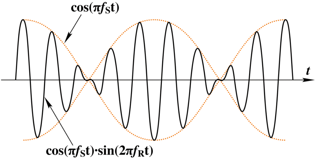
If you start with all energy in one oscillator, the energy will gradually transfer to the other oscillator and back again. The beat frequency equals the difference between the individual frequencies:
[EQUATION: f_beat = |f₁ – f₂|]
Real-World Physics: Musicians use beats to tune instruments. When two strings are nearly in tune, the beat frequency decreases toward zero as the tuning improves. Piano tuners rely on this technique to achieve precise intonation across all 88 keys.
Normal Mode Analysis: Finding the Natural Patterns
For any coupled oscillator system, normal modes represent the special oscillation patterns where all parts of the system oscillate at the same frequency with fixed phase relationships. These modes are the “building blocks” from which any possible motion can be constructed.
The mathematical analysis involves finding eigenvalues and eigenvectors of the system’s characteristic equation. For a two-oscillator system:
[EQUATION: det|k – mω² -kc | = 0]
[EQUATION: |-kc k – mω²| ]
This determinant equation yields the normal mode frequencies, while the corresponding eigenvectors describe the relative amplitudes and phases of the oscillators in each mode.
Problem-Solving Strategy: For coupled oscillator problems:
- Identify all masses and spring constants
- Write equations of motion for each oscillator
- Look for symmetric and antisymmetric solutions
- Calculate normal mode frequencies
- Use initial conditions to determine mode amplitudes
8: Laboratory Investigations and Experimental Techniques
Measuring Oscillation Parameters
Laboratory work in oscillations provides hands-on experience with fundamental physics concepts while developing crucial experimental skills. Key measurements include period determination, amplitude analysis, and energy dissipation studies.
Period Measurement Techniques:
- Stopwatch timing over multiple cycles reduces human reaction time errors
- Photogate sensors provide precise electronic timing
- Video analysis allows frame-by-frame motion study
- Computer-based data acquisition systems enable real-time analysis
Experimental Design Principle: Always measure multiple complete oscillations and divide by the number of cycles to determine the period. Single-cycle measurements introduce large uncertainties due to timing precision limitations.
Spring Constant Determination
The spring constant k can be measured using both static and dynamic methods, providing excellent opportunities to verify theoretical relationships.
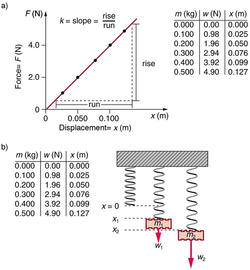
Static Method: Hang known masses from the spring and measure the resulting extensions. Plot force (mg) versus extension to find k from the slope.
Dynamic Method: Measure the oscillation period for different attached masses. Plot T² versus m; the slope equals 4π²/k.
These two independent methods should yield consistent results, providing validation of Hooke’s law and the oscillation theory.
Error Analysis Considerations:
- Spring mass affects the effective oscillating mass: m_eff = m_attached + (1/3)m_spring
- Air resistance introduces small damping effects
- Large amplitude oscillations deviate from simple harmonic behavior
- Temperature changes can affect spring properties
Pendulum Investigations
Pendulum experiments offer rich opportunities for investigating the relationships between period, length, and amplitude while exploring the limits of theoretical approximations.
Length vs. Period Investigation: Measure periods for different pendulum lengths, plotting T² versus L. The slope should equal 4π²/g, allowing determination of local gravitational acceleration.
Amplitude Effects: Investigate how period changes with amplitude, especially for larger angular displacements where the small angle approximation breaks down.
Physical Pendulum Analysis: Compare measured periods of extended objects with theoretical predictions based on moment of inertia calculations.
Real-World Connection: These same measurement principles are used in gravimeters—sensitive instruments that detect small variations in Earth’s gravitational field for geological surveying and earthquake monitoring.
Practice Problems Section: Mastering Oscillation Challenges
Multiple Choice Questions
Problem 1: A mass of 0.5 kg is attached to a spring with spring constant 200 N/m. If the mass is displaced 0.1 m from equilibrium and released, what is the maximum speed during the subsequent oscillation?
A) 1.0 m/s
B) 2.0 m/s
C) 4.0 m/s
D) 8.0 m/s
E) 16.0 m/s
Solution: Using energy conservation, the maximum kinetic energy equals the initial potential energy:
½mv²_max = ½kA²
v_max = √(kA²/m) = √(200 × 0.1²/0.5) = √4 = 2.0 m/s
Answer: B
Problem 2: Two springs with spring constants k₁ = 100 N/m and k₂ = 200 N/m are connected in series and attached to a 2.0 kg mass. What is the period of oscillation?
A) 0.21 s
B) 0.36 s
C) 0.51 s
D) 0.72 s
E) 1.02 s
Solution: For springs in series: 1/k_eff = 1/k₁ + 1/k₂ = 1/100 + 1/200 = 3/200
k_eff = 200/3 = 66.7 N/m
T = 2π√(m/k_eff) = 2π√(2.0/66.7) = 0.51 s
Answer: C
Problem 3: A simple pendulum has a period of 2.0 s on Earth (g = 9.8 m/s²). What would its period be on the Moon where g = 1.6 m/s²?
A) 0.8 s
B) 1.2 s
C) 3.2 s
D) 4.9 s
E) 6.1 s
Solution: Since T ∝ 1/√g, we have T_moon/T_earth = √(g_earth/g_moon)
T_moon = T_earth × √(9.8/1.6) = 2.0 × √6.125 = 2.0 × 2.47 = 4.9 s
Answer: D
Free Response Problems
Problem 4: A 2.0 kg block is attached to a horizontal spring with spring constant k = 800 N/m. The block is pulled 0.15 m from equilibrium and released from rest at t = 0.
a) Write expressions for the position, velocity, and acceleration as functions of time.
b) Calculate the maximum kinetic energy and maximum potential energy.
c) Find the position and velocity when the kinetic energy equals the potential energy.
d) Determine the time when the block first returns to its starting position.
Solution:
a) First find ω: ω = √(k/m) = √(800/2.0) = 20 rad/s
Since the block starts at maximum displacement and is released from rest:
x(t) = 0.15 cos(20t) m
v(t) = -3.0 sin(20t) m/s
a(t) = -60 cos(20t) m/s²
b) Maximum energies:
KE_max = ½mv²_max = ½ × 2.0 × (3.0)² = 9.0 J
PE_max = ½kA² = ½ × 800 × (0.15)² = 9.0 J
c) When KE = PE, each equals half the total energy:
KE = PE = 4.5 J
From KE = ½mv² = 4.5 J: v = ±2.12 m/s
From PE = ½kx² = 4.5 J: x = ±0.106 m
d) The block returns to x = 0.15 m when 20t = 2π
t = 2π/20 = 0.314 s
Problem 5: A uniform rod of length L = 1.0 m and mass M = 2.0 kg is pivoted at a point 0.25 m from one end and allowed to oscillate as a physical pendulum.
a) Calculate the moment of inertia about the pivot point.
b) Determine the period of small oscillations.
c) Find the length of a simple pendulum that would have the same period.
d) Explain why this length differs from the distance between the pivot and center of mass.
Solution:
a) Using the parallel axis theorem:
I_cm = (1/12)ML² = (1/12) × 2.0 × (1.0)² = 0.167 kg⋅m²
d = 0.25 m (distance from center of mass to pivot)
I_pivot = I_cm + Md² = 0.167 + 2.0 × (0.25)² = 0.292 kg⋅m²
b) For a physical pendulum:
T = 2π√(I/(Mgd)) = 2π√(0.292/(2.0 × 9.8 × 0.25)) = 1.37 s
c) For an equivalent simple pendulum:
L_equiv = T²g/(4π²) = (1.37)² × 9.8/(4π²) = 0.467 m
d) The equivalent length (0.467 m) exceeds the distance to the center of mass (0.25 m) because the rod’s distributed mass creates additional rotational inertia. The equivalent simple pendulum must be longer to account for this extra inertia while maintaining the same period.
Experimental Design Questions
Problem 6: Design an experiment to investigate how the damping coefficient affects the oscillation of a mass-spring system.
Experimental Setup:
- Vertical spring-mass system submerged in fluids of different viscosities
- High-speed camera or motion sensor for precise position tracking
- Various masses to test mass dependence
- Fluids: air, water, glycerin solutions of different concentrations
Procedure:
- Displace mass by fixed amplitude (≈ 0.05 m) and release
- Record position vs. time for at least 10 oscillation cycles
- Repeat for different fluid viscosities and different masses
- Analyze amplitude decay to determine damping coefficient γ
Data Analysis:
- Fit exponential decay envelope: A(t) = A₀e^(-γt)
- Plot ln(A) vs. t to find γ from slope
- Investigate relationship between γ and fluid viscosity
- Check if damped frequency ω’ differs significantly from natural frequency ω₀
Expected Results:
- γ should increase with fluid viscosity
- For light damping, ω’ ≈ ω₀
- Quality factor Q = ω₀/(2γ) decreases with increasing damping
Exam Preparation Strategies: Conquering the AP Physics C Oscillations Questions
Understanding AP Exam Question Types
The AP Physics C: Mechanics exam tests oscillations through several distinct question formats, each requiring specific preparation strategies.
Multiple Choice Strategies:
- Focus on conceptual understanding and quick calculations
- Master the fundamental relationships: T = 2π√(m/k) for springs, T = 2π√(L/g) for pendulums
- Practice unit analysis to eliminate incorrect answers quickly
- Memorize key values: sin(30°) = 0.5, cos(45°) = √2/2, etc.
Free Response Approaches:
- Always start by identifying the physical principles involved
- Draw clear diagrams showing forces, energy transformations, or motion patterns
- Show all algebraic work before substituting numerical values
- Include proper units and significant figures in final answers
Common Exam Mistakes and Prevention
Mistake 1: Confusing Angular Frequency with Linear Frequency
Students often mix up ω, f, and T. Remember: ω = 2πf = 2π/T
Prevention: Always check units. Angular frequency has units of rad/s, linear frequency uses Hz (s⁻¹).
Mistake 2: Forgetting the Small Angle Approximation Limitations
Simple pendulum formulas only work for small amplitudes (θ < 15°).
Prevention: Always state your approximations explicitly and check if they’re valid for the given conditions.
Mistake 3: Incorrect Energy Analysis
Students sometimes include gravitational potential energy when it’s irrelevant (horizontal oscillations) or forget it when it matters (vertical systems with changing height).
Prevention: Always identify your reference point for potential energy and be clear about which forces are conservative.
Calculator and Formula Sheet Usage
The AP Physics C exam allows programmable calculators and provides a formula sheet, but effective usage requires preparation.
Calculator Strategies:
- Program commonly used formulas and unit conversions
- Practice trigonometric calculations without looking up values
- Use graphing capabilities for analyzing oscillatory functions
- Store physical constants (g, π, etc.) in memory
Formula Sheet Mastery:
- Familiarize yourself with the exact formulas provided
- Practice deriving related formulas from the given ones
- Understand when to use each formula variation
- Know the limitations and assumptions for each formula
Conclusion and Next Steps: Your Journey Beyond Oscillations
Mastering Unit 7 of AP Physics C: Mechanics represents more than just preparing for an exam-you’ve developed a deep understanding of one of physics’ most fundamental and beautiful concepts. The principles of oscillatory motion that you’ve learned extend far beyond springs and pendulums, forming the foundation for understanding waves, quantum mechanics, electrical circuits, and countless engineering applications.
As you continue your physics journey, you’ll discover that oscillations appear everywhere: in the electromagnetic waves that carry radio signals, in the quantum mechanical wave functions that describe atomic behavior, in the thermal vibrations of atoms in solids, and in the gravitational waves recently detected from colliding black holes. The mathematical tools and physical intuition you’ve developed here will serve you well in these advanced topics.
Connecting to Future Learning
Wave Motion (if covered in your course): Oscillations are the building blocks of waves. The simple harmonic motion you’ve mastered describes how each point in a wave moves as the wave passes by.
Electricity and Magnetism: LC circuits exhibit electrical oscillations mathematically identical to mechanical spring systems, with inductance playing the role of mass and capacitance analogous to the inverse of a spring constant.
Modern Physics: Quantum harmonic oscillators describe the energy levels of atoms and molecules, while the uncertainty principle places fundamental limits on the precision of oscillation measurements.
Final Problem-Solving Wisdom
Remember that oscillation problems often have multiple solution approaches. Energy methods frequently provide the most elegant solutions, while force analysis gives deeper physical insight. Don’t hesitate to check your answers using alternative approaches when time permits.
The most successful AP Physics C students combine mathematical rigor with physical intuition. When you encounter a challenging problem, start by asking: “What physical principle governs this situation?” Then choose your mathematical tools to match the physics, not the other way around.
As you tackle the AP exam and continue your scientific education, remember that physics is ultimately about understanding the natural world. The oscillations you’ve studied govern phenomena from the atomic scale to astronomical distances, from the timing of computer processors to the stability of buildings during earthquakes. You’re not just learning equations-you’re discovering the hidden patterns that make our universe predictable, beautiful, and comprehensible.
The skills you’ve developed in analyzing oscillatory systems-breaking complex problems into manageable parts, applying fundamental principles consistently, checking results for physical reasonableness, and communicating solutions clearly-will serve you well in any scientific or technical field you choose to pursue. Whether you become a physicist, engineer, doctor, or any other professional, the analytical thinking and problem-solving approaches you’ve learned will remain valuable throughout your career.
Final Challenge: After your AP exam, try to identify oscillatory motion in your daily life. You’ll be amazed at how often these concepts apply once you know how to look for them. From the pendulum motion of walking to the acoustic oscillations that create music, the world around you is filled with the physics you’ve mastered.
Your journey in understanding oscillations is complete, but your adventure in physics is just beginning. Use the confidence and skills you’ve gained here as stepping stones to even more fascinating discoveries in the physical world. The universe is waiting for you to explore it with the tools you now possess.
Recommended –