
The Electrical World Around Us
Have you ever wondered what happens inside your smartphone when you charge it, or how electricity flows through the circuits in your home? Every time you flip a switch, plug in a device, or use any electronic gadget, you’re witnessing the principles of current electricity in action. From the microscopic movement of electrons in a copper wire to the complex circuits powering modern technology, current electricity is the invisible force that powers our digital age.
When you scroll through your phone, billions of electrons are moving through semiconductor pathways at precisely controlled rates. When you turn on an LED bulb, the same fundamental principles that govern current flow determine how efficiently electrical energy converts to light. Understanding current electricity isn’t just about passing your CBSE Class 12 Physics board exam – it’s about comprehending the technology that shapes our world.
This chapter bridges the gap between the static electrical phenomena you studied in electrostatics and the dynamic world of moving charges. You’ll discover how engineers design circuits that power everything from simple flashlights to sophisticated computers, and how the mathematical relationships you learn here form the foundation of electrical engineering.
Learning Objectives: Your Physics Journey Roadmap
By mastering CBSE Class 12 Physics Chapter 3: Current Electricity, you will achieve these essential competencies aligned with the latest 2024-25 curriculum standards:
Conceptual Mastery:
- Understand electric current as the flow of charge and relate it to everyday electrical phenomena
- Analyze the microscopic mechanism of current flow in metallic conductors through drift velocity concepts
- Comprehend the relationship between drift velocity, mobility, and current density
- Apply Ohm’s law to both ideal and real-world resistive elements
Mathematical Proficiency:
- Calculate drift velocity, current, and related quantities using fundamental equations
- Solve complex circuit problems using Kirchhoff’s voltage and current laws
- Analyze Wheatstone bridge configurations for resistance measurements
- Determine power dissipation and energy considerations in electrical circuits
Practical Applications:
- Design and analyze series and parallel resistor combinations
- Understand internal resistance effects in real batteries and cells
- Apply circuit analysis techniques to solve engineering problems
- Connect theoretical concepts to practical electrical measurements
Exam Excellence:
- Master the 17-mark weightage topics for optimal board exam performance
- Develop systematic problem-solving approaches for numerical questions
- Recognize and avoid common conceptual pitfalls in current electricity
- Apply dimensional analysis and unit consistency in electrical calculations
1. Foundation Concepts: Understanding Electric Current
Electric current forms the cornerstone of all electrical phenomena in our technological world. Unlike the stationary charges you studied in electrostatics, current electricity involves charges in motion – a dynamic process that powers everything from your calculator to electric vehicles.
Defining Electric Current
Electric current represents the rate of flow of electric charge through a cross-sectional area. When you connect a battery to a light bulb, you’re creating a pathway for electrons to flow from the negative terminal, through the circuit, and back to the positive terminal.
[EQUATION: Electric Current: I = Q/t, where I is current in amperes, Q is charge in coulombs, and t is time in seconds]
The direction of conventional current flows from positive to negative terminal (opposite to electron flow), a historical convention that remains standard in circuit analysis. This seemingly backwards convention actually simplifies mathematical analysis of circuits.
Real-World Physics: In a typical household LED bulb drawing 10 watts at 120 volts, approximately 6.25 × 10^18 electrons flow through the filament every second. That’s more electrons than there are grains of sand on Earth, all moving in coordinated fashion to produce light!
Microscopic Picture: The Journey of Electrons
Inside a metallic conductor like copper wire, electrons don’t simply race from one end to the other. Instead, they undergo a complex dance of collisions and movements that results in a net drift toward the positive terminal.
Drift Velocity: The Slow but Steady Journey
Despite electricity’s apparent instantaneous effects, individual electrons move remarkably slowly through conductors. Drift velocity represents the average velocity with which free electrons move through a conductor under the influence of an electric field.
[EQUATION: Drift Velocity: vd = I/(nAe), where vd is drift velocity, I is current, n is number density of free electrons, A is cross-sectional area, and e is electronic charge]
Physics Check: Calculate the drift velocity of electrons in a copper wire carrying 1 ampere current. With typical values (n ≈ 8.5 × 10^28 electrons/m³, A = 1 mm², e = 1.6 × 10^-19 C), you’ll find vd ≈ 0.074 mm/s – slower than a crawling ant! Yet electrical signals travel at nearly the speed of light because the electric field propagates instantaneously throughout the conductor.
Mobility: How Easily Charges Move
Mobility quantifies how quickly charge carriers respond to applied electric fields. It’s defined as the drift velocity per unit electric field:
[EQUATION: Mobility: μ = vd/E = vd/(V/L), where μ is mobility, E is electric field strength, V is potential difference, and L is length]
Higher mobility materials allow charges to move more easily, making them better conductors. Silver has the highest mobility among common metals, followed by copper and aluminum.
Common Error Alert: Students often confuse drift velocity with the speed of electrical signals. Remember: drift velocity is the slow movement of individual electrons, while electrical signals (changes in electric field) propagate at nearly light speed through the conductor.
Temperature Effects on Conductivity
As temperature increases in metals, atoms vibrate more vigorously, creating more obstacles for electron movement. This explains why electrical resistance increases with temperature in metallic conductors – a relationship crucial for understanding real-world electrical systems.
2. Ohm’s Law and Resistance: The Fundamental Relationship
Ohm’s law stands as one of physics’ most practical and widely-applied principles. Named after German physicist Georg Simon Ohm, this relationship governs virtually every electrical circuit you’ll encounter.
Understanding Ohm’s Law
Ohm’s law states that the current through a conductor is directly proportional to the potential difference across it, provided physical conditions remain constant.
[EQUATION: Ohm’s Law: V = IR, where V is potential difference (volts), I is current (amperes), and R is resistance (ohms)]
This deceptively simple equation underlies the operation of everything from simple flashlights to complex computer processors. However, Ohm’s law applies only to ohmic materials – those with linear current-voltage relationships.
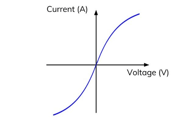
Linear vs. Non-Linear Elements
Ohmic Conductors: Materials like metals, carbon resistors, and most wire exhibit linear I-V relationships. Doubling the voltage doubles the current, maintaining constant resistance.
Non-Ohmic Elements: Semiconductors, diodes, and gas-filled tubes display non-linear I-V characteristics. LEDs, for example, conduct significantly only above a threshold voltage, then show rapid current increase.
Resistance and Resistivity: Material Properties
Resistance depends on both material properties and geometry:
[EQUATION: Resistance: R = ρL/A, where ρ is resistivity (Ω⋅m), L is length (m), and A is cross-sectional area (m²)]
Resistivity is an intrinsic material property, while resistance depends on the specific geometry of your conductor. This distinction proves crucial in engineering applications where you need to design circuits with specific resistance values.
Problem-Solving Strategy: Resistance Calculations
- Identify the geometry: Length, cross-sectional area, and material
- Look up resistivity: Use standard tables for common materials
- Apply the resistance formula: R = ρL/A
- Check units: Ensure consistency throughout calculations
- Verify reasonableness: Compare with typical values for similar conductors
Real-World Physics: The resistance of a typical household copper wire (12 AWG, 100 feet) is approximately 0.2 ohms. This seemingly small resistance can cause significant voltage drops in long extension cords, explaining why power tools sometimes run sluggishly on lengthy cords.
Temperature Dependence: Why Resistance Changes
For most metals, resistance increases linearly with temperature:
[EQUATION: Temperature Coefficient: R(T) = R₀[1 + α(T – T₀)], where α is the temperature coefficient of resistance]
This relationship explains why incandescent bulb filaments draw large initial currents (cold resistance is low) that decrease as the filament heats up. Understanding temperature effects proves essential for designing circuits that operate reliably across temperature ranges.
Historical Context: Georg Ohm faced significant resistance (pun intended) when he first published his law in 1827. The scientific community initially rejected his work, considering it too mathematical for physics. Today, his name appears on every electrical meter and circuit analysis textbook worldwide.
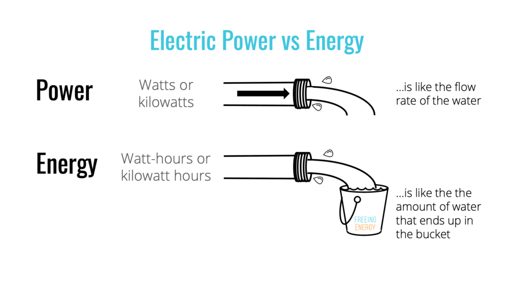
3. Electrical Power and Energy: Converting Electrical Energy
Understanding electrical power and energy consumption helps you analyze everything from battery life in portable devices to electricity bills in your home. Power represents the rate of energy transfer, while energy represents the total amount of work done by electrical forces.
Electrical Power Fundamentals
Power in electrical circuits represents the rate at which electrical energy converts to other forms – heat in resistors, light in bulbs, or mechanical work in motors.
[EQUATION: Electrical Power: P = VI = I²R = V²/R, where P is power in watts]
These three equivalent expressions prove useful in different situations. Use P = VI when you know voltage and current, P = I²R for current and resistance, and P = V²/R for voltage and resistance.
Energy and Power Consumption
Electrical energy represents the total work done over time:
[EQUATION: Electrical Energy: W = Pt = VIt, measured in joules or kilowatt-hours]
Your electricity bill calculates consumption in kilowatt-hours (kWh), where 1 kWh = 3.6 × 10⁶ joules.
Physics Check: A 100-watt bulb operating for 10 hours consumes 1 kWh of energy. At typical residential rates ($0.12/kWh), this costs about 12 cents – helping you understand energy efficiency choices.
Heat Generation in Circuits
When current flows through resistance, electrical energy converts to heat according to Joule’s law:
[EQUATION: Joule Heating: H = I²Rt, where H is heat generated in joules]
This heating effect explains why electrical components have power ratings and why proper cooling is essential in electronic devices. Excessive heating can damage components or create fire hazards.
Efficiency Considerations
Real circuits involve energy losses, primarily through resistive heating. Efficiency quantifies useful power output versus total power input:
[EQUATION: Efficiency: η = (Useful Power Output)/(Total Power Input) × 100%]
Power transmission systems use high voltages to minimize current (and thus I²R losses) over long distances, then step down voltage for safe household use.
4. Series and Parallel Circuits: Building Complex Networks
Understanding series and parallel combinations forms the foundation for analyzing any complex electrical circuit. These basic configurations appear in every electronic device, from simple flashlights to sophisticated computers.
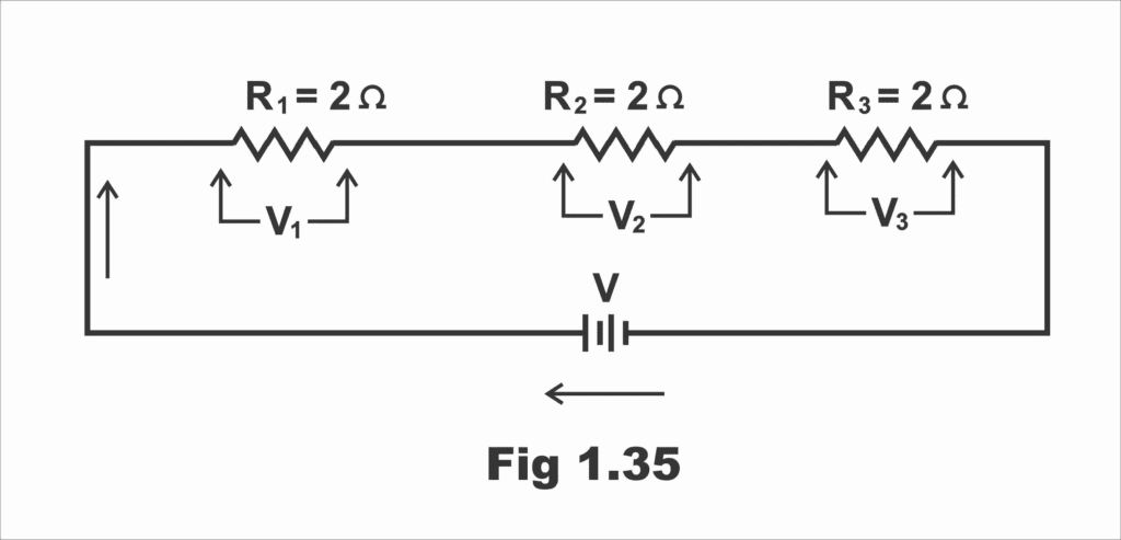
Series Circuits: Single Path Analysis
In series circuits, components connect end-to-end, creating a single path for current flow. This configuration appears in holiday lights, some car headlights, and various control circuits.
Series Circuit Properties:
- Current remains constant throughout: I₁ = I₂ = I₃ = I_total
- Voltages add: V_total = V₁ + V₂ + V₃
- Resistances add: R_total = R₁ + R₂ + R₃
[EQUATION: Series Resistance: R_eq = R₁ + R₂ + R₃ + … + Rₙ]
Real-World Physics: Old Christmas lights used series connections. When one bulb burned out, the entire string went dark because the circuit path was broken. Modern LED strings use parallel connections with series sections to prevent this problem while maintaining energy efficiency.
Parallel Circuits: Multiple Path Analysis
Parallel circuits provide multiple pathways for current flow. This configuration appears in household wiring, car electrical systems, and computer circuits.
Parallel Circuit Properties:
- Voltage remains constant across branches: V₁ = V₂ = V₃ = V_total
- Currents add: I_total = I₁ + I₂ + I₃
- Reciprocal resistances add: 1/R_total = 1/R₁ + 1/R₂ + 1/R₃
[EQUATION: Parallel Resistance: 1/R_eq = 1/R₁ + 1/R₂ + 1/R₃ + … + 1/Rₙ]
Problem-Solving Strategy: Complex Circuit Analysis
- Identify series and parallel sections: Start from the source and trace current paths
- Calculate equivalent resistances: Combine resistors step by step
- Work backward: Use Ohm’s law to find currents and voltages
- Verify results: Check that power dissipated equals power supplied
- Apply Kirchhoff’s laws: Ensure current and voltage conservation
Common Error Alert: When calculating parallel resistance, remember that the equivalent resistance is always less than the smallest individual resistance. Many students incorrectly add parallel resistances directly instead of using the reciprocal formula.
5. Kirchhoff’s Laws: Advanced Circuit Analysis
While Ohm’s law governs individual components, Kirchhoff’s laws govern entire circuits. These powerful principles, formulated by German physicist Gustav Kirchhoff, enable analysis of any circuit configuration, no matter how complex.
Kirchhoff’s Current Law (KCL): Conservation of Charge
KCL states that the algebraic sum of currents entering any junction equals zero. This reflects charge conservation – charge cannot accumulate at any point in a steady-state circuit.
[EQUATION: KCL: Σ I_entering = Σ I_leaving, or Σ I = 0 at any junction]
Practical Application: At any circuit node, assign positive signs to currents entering and negative signs to currents leaving. The algebraic sum must equal zero.
Kirchhoff’s Voltage Law (KVL): Conservation of Energy
KVL states that the algebraic sum of potential differences around any closed loop equals zero. This reflects energy conservation – you cannot gain or lose energy by moving charge around a closed path.
[EQUATION: KVL: Σ V = 0 around any closed loop]
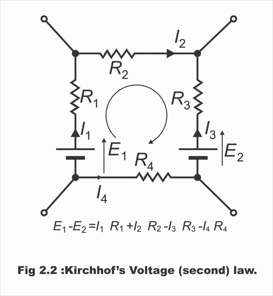
Advanced Problem-Solving: Mesh Analysis
For complex circuits with multiple sources and resistors, mesh analysis provides systematic solution methods:
- Identify independent loops: Choose mesh currents for each loop
- Apply KVL: Write voltage equations for each mesh
- Solve simultaneously: Use algebraic methods to find mesh currents
- Calculate branch currents: Combine mesh currents as needed
Real-World Physics: Circuit analysis software used in engineering (like SPICE) fundamentally applies Kirchhoff’s laws with matrix mathematics to solve circuits containing thousands of components. Your smartphone’s processor design relies on these same principles applied to circuits with billions of transistors.
Historical Context: Gustav Kirchhoff developed these laws while still a university student in 1845. His mathematical approach to circuit analysis revolutionized electrical engineering and remains the foundation of modern circuit design software.
6. Internal Resistance and EMF: Real Battery Behavior
Ideal voltage sources maintain constant voltage regardless of current drawn. Real batteries and power supplies exhibit internal resistance that affects their terminal voltage under load. Understanding this behavior proves crucial for designing reliable circuits and predicting battery performance.
Electromotive Force (EMF) Concepts
EMF represents the energy per unit charge provided by a battery or generator, measured when no current flows (open-circuit voltage). This differs from terminal voltage, which decreases when current is drawn.
[EQUATION: Terminal Voltage: V = ℰ – Ir, where ℰ is EMF, I is current, and r is internal resistance]
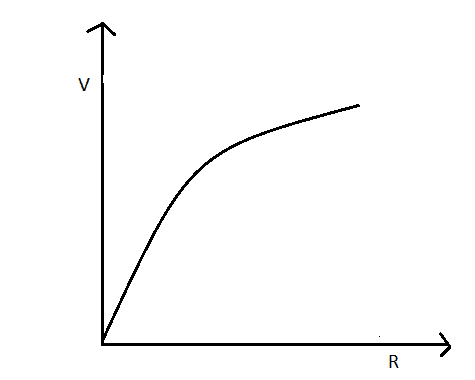
Battery Performance Analysis
Real batteries exhibit internal resistance that increases with age, temperature effects, and discharge state. This explains why car batteries struggle in cold weather and why flashlight bulbs dim as batteries drain.
Battery Performance Graph:
Maximum Power Transfer
For any circuit with internal resistance, maximum power transfers to the load when load resistance equals internal resistance:
[EQUATION: Maximum Power Transfer: R_load = r_internal for maximum power]
However, maximum efficiency occurs when load resistance is much larger than internal resistance, creating a design trade-off between power and efficiency.
Problem-Solving Strategy: Internal Resistance Problems
- Identify EMF and internal resistance: Use given values or calculate from open/short circuit conditions
- Calculate total resistance: R_total = R_external + r_internal
- Find circuit current: I = ℰ/R_total
- Determine terminal voltage: V = ℰ – Ir
- Calculate power distributions: Between internal and external resistances
Real-World Physics: Smartphone batteries exhibit internal resistance that increases as they age. This explains why older phones may shut down unexpectedly under high processor loads – the internal resistance causes voltage to drop below the minimum required for stable operation.
7. Combination of Cells: Power Supply Design
Multiple cells can be combined in various configurations to achieve desired voltage and current capabilities. Understanding these combinations helps you design power supplies for specific applications and understand battery pack behavior in devices from laptops to electric vehicles.
Series Combination of Cells
Connecting cells in series adds their EMFs while maintaining the same current capability:
[EQUATION: Series Cells: ℰ_total = ℰ₁ + ℰ₂ + ℰ₃, r_total = r₁ + r₂ + r₃]
This configuration appears in flashlights, where multiple 1.5V cells create higher voltage for brighter bulbs.
Parallel Combination of Cells
Parallel connection maintains EMF while reducing effective internal resistance and increasing current capability:
[EQUATION: Parallel Cells: ℰ_total = ℰ (same for identical cells), 1/r_total = 1/r₁ + 1/r₂ + 1/r₃]
Mixed Combinations: Series-Parallel Arrays
Complex battery packs use series-parallel combinations to achieve both higher voltage and current capabilities. Laptop batteries typically use this configuration to provide 10-15V at several amperes.
Real-World Physics: Electric vehicle battery packs contain thousands of small cells arranged in complex series-parallel combinations. Tesla Model S batteries contain over 7,000 individual lithium-ion cells configured to provide 400V at hundreds of amperes – enough power to accelerate a 2-ton car from 0-60 mph in under 3 seconds.
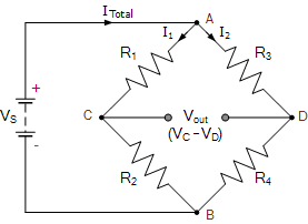
8. Wheatstone Bridge: Precision Resistance Measurement
The Wheatstone bridge represents one of the most elegant and precise methods for measuring unknown resistances. This circuit configuration, perfected by Sir Charles Wheatstone, enables resistance measurements with extraordinary accuracy and forms the basis for many electronic sensors.
Wheatstone Bridge Principles
A Wheatstone bridge consists of four resistors arranged in a diamond configuration with a galvanometer connecting opposite corners. When the bridge is balanced, no current flows through the galvanometer.
[EQUATION: Balance Condition: R₁/R₂ = R₃/R₄, or R₁R₄ = R₂R₃]
Applications and Variations
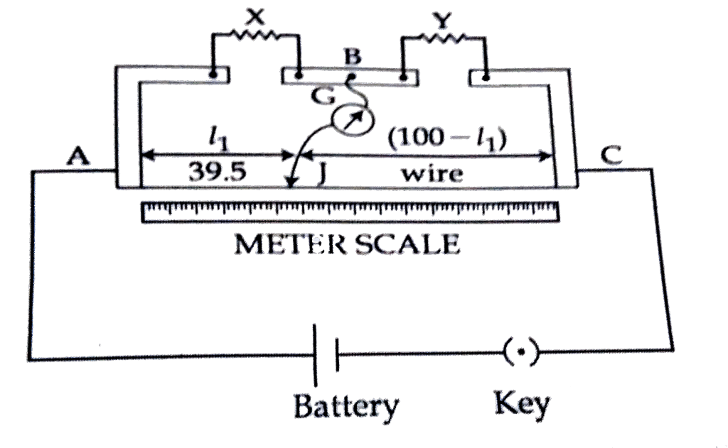
Meter Bridge: A practical implementation using a uniform wire and sliding contact, allowing precise resistance measurement through length measurements.
Strain Gauges: Use the bridge principle to detect tiny resistance changes caused by mechanical deformation, enabling precise force and pressure measurements.
Temperature Sensors: Resistance thermometers (RTDs) use bridge circuits to detect temperature-induced resistance changes with high precision.
Problem-Solving Strategy: Bridge Analysis
- Check balance condition: Determine if R₁R₄ = R₂R₃
- For balanced bridges: No current through galvanometer; calculate other branch currents
- For unbalanced bridges: Use Kirchhoff’s laws to analyze complete network
- Sensitivity analysis: Determine how small resistance changes affect galvanometer current
Real-World Physics: Modern electronic scales use strain gauge bridges to measure weight. When you step on the scale, tiny deflections in the platform create resistance changes in the bridge circuit. These changes, measured with precision electronics, translate directly to weight measurements accurate to fractions of a pound.
9. Experimental Investigations: Laboratory Applications
Current electricity concepts come alive through hands-on laboratory investigations. These experiments not only reinforce theoretical understanding but also develop practical skills essential for any scientific or engineering career.
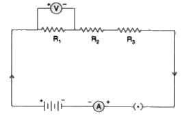
Ohm’s Law Verification Experiment
Objective: Verify the linear relationship between voltage and current for ohmic materials.
Procedure: Use a variable DC power supply, ammeter, voltmeter, and known resistors to measure I-V characteristics across different voltage ranges.
Key Measurements:
- Record voltage and current pairs for various settings
- Plot V vs. I graphs for different resistors
- Calculate resistance from slope and compare with nominal values
- Analyze deviations from linearity at high currents
Error Analysis: Consider systematic errors from meter accuracy, contact resistance, and thermal effects. Random errors arise from meter reading limitations and environmental fluctuations.
Wheatstone Bridge Investigation
Setup: Use a meter bridge apparatus with known and unknown resistors, galvanometer, and jockey for balance point detection.
Measurements:
- Find balance points for various resistance ratios
- Calculate unknown resistances using the balance condition
- Investigate sensitivity by measuring galvanometer deflection for small resistance changes
- Study temperature effects on wire resistance
Real-World Extension: Connect strain gauges or thermistors to observe bridge applications in sensor technology.
Kirchhoff’s Laws Verification
Circuit Construction: Build networks with multiple resistors and voltage sources to test current and voltage conservation.
Verification Process:
- Measure all branch currents and verify KCL at junctions
- Measure voltages around closed loops and verify KVL
- Compare measured values with theoretical predictions
- Analyze sources of discrepancy
Safety Considerations
Always follow proper laboratory safety protocols:
- Check circuit connections before applying power
- Use appropriate voltage and current ratings for all components
- Never exceed component power ratings
- Handle meters and instruments carefully to maintain calibration
Data Analysis Techniques
Graph Analysis: Linear regression for I-V plots helps determine resistance values and assess linearity.
Uncertainty Propagation: Calculate uncertainties in derived quantities using proper error analysis methods.
Statistical Analysis: Multiple measurements enable calculation of mean values and standard deviations.
Practice Problems Section: Master Your Skills
Multiple Choice Questions (MCQs)
Problem 1: The drift velocity of electrons in a copper wire carrying 2A current with cross-sectional area 2 mm² is approximately (given: n = 8.5 × 10²⁸ m⁻³, e = 1.6 × 10⁻¹⁹ C):
A) 0.074 mm/s B) 0.148 mm/s C) 0.037 mm/s D) 0.296 mm/s
Solution: Using vd = I/(nAe)
vd = 2/(8.5 × 10²⁸ × 2 × 10⁻⁶ × 1.6 × 10⁻¹⁹)
vd = 2/(27.2 × 10³) = 0.074 × 10⁻³ m/s = 0.074 mm/s
Answer: A
Problem 2: A wire has resistance R. If it’s stretched to double its length, the new resistance becomes:
A) R/4 B) R/2 C) 2R D) 4R
Solution: When length doubles, cross-sectional area halves (constant volume).
Using R = ρL/A, new resistance = ρ(2L)/(A/2) = 4ρL/A = 4R
Answer: D
Problem 3: In a Wheatstone bridge, if R₁ = 10Ω, R₂ = 20Ω, R₃ = 30Ω, the value of R₄ for balance is:
A) 40Ω B) 50Ω C) 60Ω D) 70Ω
Solution: Balance condition: R₁/R₂ = R₃/R₄
10/20 = 30/R₄
R₄ = 30 × 20/10 = 60Ω
Answer: C
Numerical Problems with Complete Solutions
Problem 4: A battery with EMF 12V and internal resistance 0.5Ω is connected to an external resistance of 3.5Ω. Calculate:
a) Current in the circuit
b) Terminal voltage
c) Power dissipated in external resistance
d) Efficiency of the battery
Solution:
Given: ℰ = 12V, r = 0.5Ω, R = 3.5Ω
a) Current: I = ℰ/(R + r) = 12/(3.5 + 0.5) = 12/4 = 3A
b) Terminal voltage: V = ℰ – Ir = 12 – (3)(0.5) = 12 – 1.5 = 10.5V
c) Power in external resistance: P_ext = I²R = (3)²(3.5) = 31.5W
d) Efficiency: η = P_ext/P_total = (I²R)/(I²(R+r)) = R/(R+r) = 3.5/4 = 87.5%
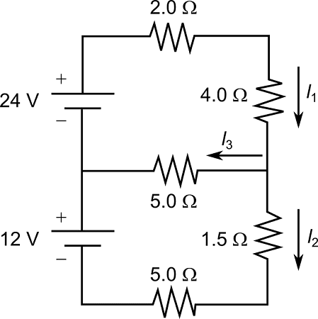
Problem 5: In the circuit shown, find the current through each resistor using Kirchhoff’s laws.
Solution using mesh analysis:
Step 1: Define mesh currents I₁ (left loop) and I₂ (right loop)
Step 2: Apply KVL to each mesh:
Left mesh: 10 – 2I₁ – 4(I₁ – I₂) = 0
Simplifying: 10 – 6I₁ + 4I₂ = 0 …(1)
Right mesh: 6 – 3I₂ – 4(I₂ – I₁) = 0
Simplifying: 6 – 7I₂ + 4I₁ = 0 …(2)
Step 3: Solve simultaneously:
From equation (1): 4I₂ = 6I₁ – 10
I₂ = 1.5I₁ – 2.5
Substituting in equation (2):
6 – 7(1.5I₁ – 2.5) + 4I₁ = 0
6 – 10.5I₁ + 17.5 + 4I₁ = 0
23.5 – 6.5I₁ = 0
I₁ = 23.5/6.5 = 3.62A
I₂ = 1.5(3.62) – 2.5 = 2.93A
Step 4: Calculate branch currents:
- Through 2Ω resistor: I₁ = 3.62A
- Through 3Ω resistor: I₂ = 2.93A
- Through 4Ω resistor: I₁ – I₂ = 3.62 – 2.93 = 0.69A
Advanced Problem-Solving Challenges
Problem 6: A potentiometer wire of length 100 cm has resistance 10Ω. It is connected to a 2V battery. An unknown EMF is balanced at 60 cm from the positive terminal. If a 2Ω resistor is connected across the unknown EMF, the balance point shifts to 50 cm. Find the unknown EMF and its internal resistance.
Solution:
Step 1: Calculate potential gradient
Potential gradient = V/L = 2V/100cm = 0.02 V/cm
Step 2: Find unknown EMF
Without external load: ℰ = potential gradient × balance length
ℰ = 0.02 × 60 = 1.2V
Step 3: Analyze circuit with external load
With 2Ω load, terminal voltage = 0.02 × 50 = 1.0V
Step 4: Apply internal resistance relationship
Terminal voltage = ℰ – I_load × r
Where I_load = ℰ/(R_load + r) = 1.2/(2 + r)
1.0 = 1.2 – [1.2/(2 + r)] × r
1.0 = 1.2 – 1.2r/(2 + r)
1.0(2 + r) = 1.2(2 + r) – 1.2r
2 + r = 2.4 + 1.2r – 1.2r
2 + r = 2.4
r = 0.4Ω
Answer: Unknown EMF = 1.2V, Internal resistance = 0.4Ω
Conceptual Application Problems
Problem 7: Explain why household appliances are connected in parallel rather than series, and calculate the total current drawn when a 100W bulb, 1500W microwave, and 800W toaster operate simultaneously on 120V supply.
Solution:
Parallel Connection Advantages:
- Independent operation: Each device can be controlled separately
- Constant voltage: Each device receives full supply voltage
- Failure isolation: One device failure doesn’t affect others
- Power ratings maintained: Devices operate at designed power levels
Current Calculations:
Using P = VI, so I = P/V
- Bulb current: I₁ = 100W/120V = 0.83A
- Microwave current: I₂ = 1500W/120V = 12.5A
- Toaster current: I₃ = 800W/120V = 6.67A
Total current: I_total = I₁ + I₂ + I₃ = 0.83 + 12.5 + 6.67 = 20.0A
This explains why circuit breakers typically rate at 15-20A for household circuits.
Data Analysis Problems
Problem 8: In a temperature coefficient experiment, a wire’s resistance varies as shown:
Temperature (°C): 20, 40, 60, 80, 100
Resistance (Ω): 100.0, 107.8, 115.6, 123.4, 131.2
Calculate the temperature coefficient of resistance and predict resistance at 150°C.
Solution:
Step 1: Use linear relationship R(T) = R₀[1 + α(T – T₀)]
Step 2: Calculate temperature coefficient
Using two points: (20°C, 100Ω) and (100°C, 131.2Ω)
131.2 = 100[1 + α(100 – 20)]
1.312 = 1 + 80α
α = 0.312/80 = 0.0039/°C
Step 3: Verify with other data points
At 60°C: R = 100[1 + 0.0039(60-20)] = 100[1 + 0.156] = 115.6Ω ✓
Step 4: Predict at 150°C
R(150) = 100[1 + 0.0039(150-20)] = 100[1 + 0.507] = 150.7Ω
Answer: Temperature coefficient α = 0.0039/°C, R(150°C) = 150.7Ω
Frequent 3-5 Mark Problems:
Memory Techniques:
- Use acronyms for Kirchhoff’s laws: “Current Can’t Collect” (KCL), “Voltage Vanishes in Loops” (KVL)
- Create formula sheets with derivation steps
- Practice drawing circuits from memory
- Associate equations with real-world examples
Conclusion: Your Path to Physics Excellence
Mastering current electricity opens doors to understanding virtually all modern technology. From the smartphone in your pocket to the power grid supplying your home, the principles you’ve learned here govern the flow of electrical energy that powers our digital age.
Your journey through current electricity has equipped you with both mathematical tools and conceptual understanding. You can now analyze circuits with confidence, predict battery behavior, understand why devices are wired as they are, and appreciate the elegant physics behind electrical measurements. These skills extend far beyond exam success = they form the foundation for careers in electrical engineering, electronics, renewable energy, and countless technology fields.
Looking Forward: Current electricity concepts directly connect to upcoming chapters on magnetism, electromagnetic induction, and AC circuits. Your solid foundation here will make these advanced topics much more accessible and intuitive.
Remember that physics is fundamentally about understanding how nature works. Every equation represents a deep truth about electrical phenomena, every circuit analysis reveals the elegant logic of charge and energy conservation. As you prepare for your exams, maintain this sense of wonder about the physical world – it will serve you well whether you pursue physics further or apply these concepts in engineering, technology, or everyday problem-solving.
Your mastery of current electricity represents more than academic achievement; it’s your entry point into the technological literacy essential for 21st-century success. The same principles governing your study circuits will help you understand emerging technologies like electric vehicles, renewable energy systems, and advanced electronics throughout your career.
The physics of current electricity surrounds us constantly. Every time you flip a switch, charge a device, or use any electrical appliance, you’re witnessing these principles in action. Your deep understanding of these concepts will serve as a foundation for lifelong learning and success in our increasingly technological world.
About Solveify AI: Your trusted partner for comprehensive CBSE board exam preparation, offering expert-crafted study materials, detailed solutions, and strategic exam guidance for academic excellence.
Your Success Mantra:
“Current flows, voltage drops, energy conserves – and I understand it all!”
Recommended –
1 thought on “CBSE Class 12 Physics Chapter 3: Current Electricity – Complete Study Guide 2025-26”