AP Physics C: Mechanics Unit 1 Kinematics – Ultimate 2025 Study Guide | Equations, Problems & Tips

The Physics of Everything That Moves

Every morning when you check your phone, you’re witnessing kinematics in action. The smooth scrolling motion across your screen, the way your car accelerates from a stoplight, even the path of a basketball arcing through the air – all of these everyday phenomena follow the precise mathematical relationships you’ll master in AP Physics C: Mechanics Unit 1 Kinematics.

Kinematics, derived from the Greek word “kinema” meaning movement, is the branch of physics that describes motion without considering the forces that cause it. Think of it as the grammar of motion – before you can understand why objects move the way they do, you need to develop a precise vocabulary for describing how they move.

Unlike the algebra-based AP Physics 1, AP Physics C: Mechanics uses calculus to unlock deeper insights into motion. This mathematical sophistication allows you to analyze complex real-world scenarios that would be impossible to solve with basic algebraic methods. From designing roller coasters to programming autonomous vehicles, the concepts you’ll learn form the foundation of modern engineering and technology.

This comprehensive study guide will transform you from a student who memorizes kinematic equations into someone who truly understands the elegant mathematical relationships governing motion. You’ll discover how position, velocity, and acceleration are connected through calculus, learn to solve complex motion problems with confidence, and develop the analytical skills essential for success on the AP Physics C: Mechanics exam.

Learning Objectives: Your Roadmap to Kinematic Mastery

By the end of this unit, you will demonstrate mastery of College Board’s essential learning objectives for AP Physics C: Mechanics kinematics:

Conceptual Understanding:

• Analyze motion in one and two dimensions using position, velocity, and acceleration vectors
• Distinguish between average and instantaneous quantities using calculus-based definitions
• Interpret graphical representations of motion and extract quantitative information
• Apply kinematic principles to projectile motion and relative motion scenarios

Mathematical Proficiency:

• Use derivatives to find velocity from position functions and acceleration from velocity functions
• Apply integration to determine position from velocity and velocity from acceleration
• Solve differential equations representing motion under constant and variable acceleration
• Perform vector analysis for two-dimensional motion problems

Problem-Solving Skills:

• Select appropriate kinematic models for various motion scenarios
• Design and analyze experiments to investigate motion relationships
• Evaluate the reasonableness of solutions through dimensional analysis and limiting cases
• Connect kinematic descriptions to real-world engineering and physics applications

1: Foundations of Motion Analysis

Understanding Position, Displacement, and Coordinate Systems

Position serves as the fundamental building block of all kinematic analysis. In AP Physics C, we define position as a vector quantity that specifies an object’s location relative to a chosen coordinate system. Unlike everyday language where “position” might be vague, physics demands mathematical precision.

Consider a car traveling along a straight highway. If we establish our coordinate system with the origin at mile marker zero and the positive x-direction pointing east, then a car located at mile marker 15 has a position vector of +15 miles. This seems straightforward, but the real power emerges when we consider how position changes with time.

Displacement represents the change in position between two moments in time. Mathematically, we express this as:

[EQUATION: Δx = x₂ – x₁, where Δx represents displacement, x₂ is final position, and x₁ is initial position]

The vector nature of displacement becomes crucial in multi-dimensional problems. A hiker who walks 3 km north, then 4 km east, has traveled a total distance of 7 km but experienced a displacement of 5 km in the northeast direction. This distinction between distance (a scalar) and displacement (a vector) appears frequently on AP exam questions.

Real-World Physics: GPS Navigation

Modern GPS systems rely heavily on kinematic principles to track your location and predict arrival times. Your smartphone continuously calculates position vectors relative to satellite coordinates, then uses calculus-based algorithms to determine your velocity and predict future positions. The “estimated time of arrival” feature essentially solves kinematic equations in real-time, accounting for variable speeds and route changes.

2: Velocity – The Rate of Motion

From Average to Instantaneous Velocity

Velocity quantifies how quickly position changes with time. While this concept seems intuitive, the calculus-based approach in AP Physics C reveals subtle but important distinctions that don’t appear in algebra-based courses.

Average velocity over a time interval provides useful information but masks important details about motion:

[EQUATION: v̄ = Δx/Δt = (x₂ – x₁)/(t₂ – t₁), representing average velocity as total displacement divided by elapsed time]

However, instantaneous velocity – the velocity at a specific moment – requires calculus. As we make the time interval infinitesimally small, average velocity approaches instantaneous velocity:

[EQUATION: v(t) = lim(Δt→0) Δx/Δt = dx/dt, defining instantaneous velocity as the derivative of position with respect to time]

This mathematical relationship reveals a profound connection: velocity is the first derivative of position. This isn’t just abstract mathematics – it’s the foundation for understanding how motion unfolds in real time.

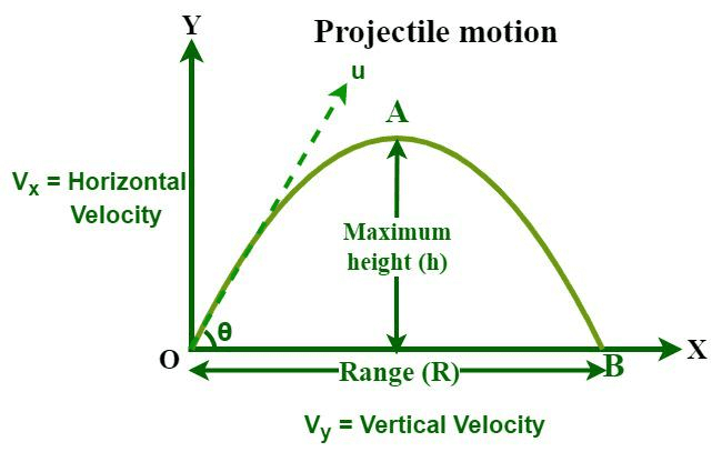
Interpreting Position-Time Graphs

Position-time graphs provide visual representations of motion that often appear on AP exam questions. The slope of a position-time graph at any point equals the instantaneous velocity at that moment. This graphical interpretation connects calculus concepts to visual analysis.

When analyzing position-time graphs, look for these key features:

• Horizontal segments indicate zero velocity (object at rest)
• Positive slopes represent motion in the positive direction
• Negative slopes indicate motion in the negative direction
• Curved lines suggest changing velocity (acceleration present)
• The steepness of the curve indicates the magnitude of velocity

Physics Check: Velocity Concepts

Test your understanding with this scenario: A particle’s position is described by x(t) = 3t² – 2t + 1, where x is in meters and t is in seconds. What is the particle’s velocity at t = 2 seconds?

Solution: v(t) = dx/dt = 6t – 2. At t = 2 seconds, v(2) = 6(2) – 2 = 10 m/s.

3: Acceleration – The Dynamics of Velocity Change

Defining Acceleration Through Calculus

Acceleration describes how velocity changes with time. Just as velocity represents the rate of change of position, acceleration represents the rate of change of velocity:

[EQUATION: a(t) = dv/dt = d²x/dt², showing acceleration as both the derivative of velocity and the second derivative of position]

This double derivative relationship provides powerful analytical tools for solving complex motion problems. Unlike constant acceleration scenarios you might remember from earlier physics courses, AP Physics C prepares you to handle variable acceleration situations common in advanced applications.

Average acceleration follows a similar pattern to average velocity:

[EQUATION: ā = Δv/Δt = (v₂ – v₁)/(t₂ – t₁), representing average acceleration as change in velocity divided by time interval]

The vector nature of acceleration creates interesting possibilities. An object can have constant speed but changing velocity if its direction changes – think of uniform circular motion. Conversely, an object moving in a straight line experiences acceleration only when its speed changes.

Velocity-Time Graph Analysis

Velocity-time graphs reveal acceleration information through their slopes, just as position-time graphs reveal velocity through their slopes. This creates a hierarchical relationship among kinematic quantities that appears frequently in AP exam problems.

Key features to identify in velocity-time graphs:

• Horizontal lines indicate constant velocity (zero acceleration)
• Straight sloped lines represent constant acceleration
• Curved lines suggest variable acceleration
• The area under the curve represents displacement

Common Error Alert: Signs and Directions

Students frequently confuse negative acceleration with “slowing down.” Remember that acceleration direction depends on your chosen coordinate system, not on whether the object is speeding up or slowing down. An object moving in the negative direction while experiencing negative acceleration is actually speeding up, not slowing down.

4: Mathematical Framework – The Kinematic Equations

Deriving Equations from First Principles

The standard kinematic equations that you may have memorized in previous courses can be derived from calculus, providing deeper insight into their origins and limitations. Let’s explore how these familiar relationships emerge from fundamental definitions.

Starting with constant acceleration, we know that a = dv/dt = constant. Integrating both sides:

[EQUATION: ∫dv = ∫a dt, which gives us v(t) = at + C, where C is the integration constant]

Using initial conditions (v = v₀ when t = 0), we find C = v₀, yielding:

[EQUATION: v(t) = v₀ + at, the fundamental velocity equation for constant acceleration]

Similarly, since v = dx/dt, we can integrate again:

[EQUATION: ∫dx = ∫(v₀ + at)dt, resulting in x(t) = v₀t + ½at² + C]

With initial conditions (x = x₀ when t = 0), we obtain:

[EQUATION: x(t) = x₀ + v₀t + ½at², the fundamental position equation for constant acceleration]

These derivations reveal why kinematic equations work and, equally important, when they don’t apply. The constant acceleration assumption is crucial – these equations become invalid when acceleration varies with time.

The Complete Kinematic Toolkit

For constant acceleration motion, you have five primary equations at your disposal:

[EQUATION: v = v₀ + at (velocity as a function of time)] [EQUATION: x = x₀ + v₀t + ½at² (position as a function of time)] [EQUATION: v² = v₀² + 2a(x – x₀) (velocity-position relationship)] [EQUATION: x = x₀ + ½(v₀ + v)t (average velocity approach)] [EQUATION: x = x₀ + vt – ½at² (alternative position equation)]

Each equation contains four of the five kinematic variables (x, x₀, v, v₀, a, t). Choose the equation that includes three known quantities and the one unknown you need to find.

Problem-Solving Strategy: The GUESS Method

Successful kinematic problem solving follows a systematic approach:

G – Given: List all known quantities with proper units U – Unknown: Identify what you need to find E – Equation: Select the appropriate kinematic equation S – Substitute: Insert known values and solve S – Sense-check: Verify your answer is reasonable

This methodical approach prevents common errors and builds confidence in complex problems.

5: One-Dimensional Motion Applications

Free Fall Analysis

Free fall motion provides an excellent application of kinematic principles because acceleration remains constant (g = 9.8 m/s² downward near Earth’s surface). However, AP Physics C problems often include complications that require careful analysis.

Consider an object thrown upward with initial velocity v₀. The complete motion analysis requires understanding that acceleration remains constant throughout the flight, even when the object momentarily stops at maximum height.

At maximum height, velocity equals zero, but acceleration still equals -g. This counterintuitive result often appears in exam questions. Many students incorrectly assume that zero velocity implies zero acceleration.

Real-World Physics: Skydiving and Terminal Velocity

While introductory free fall problems assume constant acceleration, real falling objects eventually reach terminal velocity when air resistance balances gravitational force. Professional skydivers manipulate their body position to control terminal velocity, reaching speeds around 55 m/s (120 mph) in belly-to-earth position or over 90 m/s (200 mph) in head-down orientation. These scenarios require more advanced analysis involving variable acceleration.

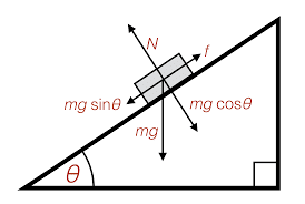
Motion Along Inclined Planes

Inclined plane problems combine one-dimensional kinematics with basic force analysis. When an object moves along a frictionless incline, its acceleration equals g sin θ, where θ represents the angle from horizontal.

[EQUATION: a = g sin θ (acceleration down a frictionless incline)]

This relationship demonstrates how kinematics connects to dynamics – the acceleration depends on the component of gravitational force parallel to the incline surface.

Physics Check: Inclined Plane Motion

A ball rolls down a frictionless incline that makes a 30° angle with horizontal. If the ball starts from rest and travels 5.0 meters along the incline, what is its final velocity?

Solution: Given: θ = 30°, x₀ = 0, v₀ = 0, x = 5.0 m Unknown: v First find acceleration: a = g sin 30° = 9.8 × 0.5 = 4.9 m/s² Use v² = v₀² + 2a(x – x₀): v² = 0 + 2(4.9)(5.0) = 49 Therefore: v = 7.0 m/s

6: Two-Dimensional Motion and Projectile Motion

Vector Analysis in Kinematics

Two-dimensional motion requires vector analysis skills that distinguish AP Physics C from simpler courses. Position, velocity, and acceleration all become vector quantities with independent horizontal and vertical components.

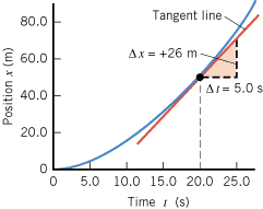
The key insight for projectile motion is that horizontal and vertical motions are independent. Gravity affects only vertical motion, leaving horizontal motion unchanged (ignoring air resistance). This principle, known as the independence of perpendicular motions, simplifies complex trajectories into manageable one-dimensional problems.

[EQUATION: x-direction: vₓ = v₀ₓ = constant, x = x₀ + v₀ₓt] [EQUATION: y-direction: vᵧ = v₀ᵧ – gt, y = y₀ + v₀ᵧt – ½gt²]

Analyzing Projectile Trajectories

The trajectory equation for projectile motion combines horizontal and vertical motion descriptions. By eliminating time from the parametric equations, we obtain:

[EQUATION: y = y₀ + x tan θ – (gx²)/(2v₀² cos² θ), describing the parabolic path of projectile motion]

This equation reveals the parabolic nature of projectile paths and allows direct calculation of trajectory properties without time-based analysis.

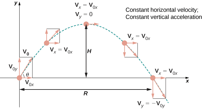
Range and Maximum Height Calculations

For projectiles launched from ground level, maximum range occurs at 45° launch angle:

[EQUATION: R = (v₀² sin 2θ)/g (range equation for projectile motion)]

Maximum height depends only on vertical launch velocity:

[EQUATION: h = (v₀ sin θ)²/(2g) (maximum height equation)]

These relationships demonstrate how launch angle affects trajectory characteristics, information crucial for applications ranging from sports to spacecraft trajectories.

Problem-Solving Strategy: Component Analysis

Complex projectile problems become manageable when you systematically analyze each component:

1. Establish coordinate system with appropriate origin
2. Resolve initial velocity into horizontal and vertical components
3. Apply kinematic equations separately to each direction
4. Combine results to find final answers

This approach works for any projectile motion scenario, from simple parabolic paths to complex multi-stage trajectories.

7: Relative Motion and Reference Frames

Understanding Reference Frame Dependencies

Motion descriptions depend entirely on your chosen reference frame. A passenger on a train moving at constant velocity observes different motion than a stationary observer on the ground. AP Physics C problems often require analyzing motion from multiple reference frames.

The velocity addition formula for relative motion states:

[EQUATION: v⃗ₐ = v⃗ₐ/ᵦ + v⃗ᵦ, where v⃗ₐ is velocity of A relative to ground, v⃗ₐ/ᵦ is velocity of A relative to B, and v⃗ᵦ is velocity of B relative to ground]

This vector equation requires careful attention to direction and coordinate systems, especially in two-dimensional problems.

River Crossing Problems

Classic relative motion scenarios involve boats crossing rivers with currents. The boat’s velocity relative to water combines vectorially with the water’s velocity relative to ground to determine the boat’s velocity relative to ground.

These problems test your understanding of vector addition and often require optimization strategies to minimize crossing time or drift distance.

Real-World Physics: Aircraft Navigation

Commercial aircraft constantly deal with relative motion as they navigate through moving air masses. Pilots must account for wind velocity when planning flight paths, calculating fuel requirements, and determining arrival times. GPS systems provide ground velocity while airspeed indicators show velocity relative to surrounding air.

8: Calculus Applications in Advanced Kinematics

Variable Acceleration Analysis

Real-world motion often involves changing acceleration, requiring calculus methods beyond the standard kinematic equations. When acceleration varies with time, position, or velocity, you must return to fundamental derivative and integral relationships.

For acceleration as a function of time, a(t):

[EQUATION: v(t) = v₀ + ∫₀ᵗ a(t’)dt’ (velocity from time-dependent acceleration)] [EQUATION: x(t) = x₀ + ∫₀ᵗ v(t’)dt’ (position from velocity function)]

These integrals may require advanced calculus techniques depending on the acceleration function’s complexity.

Position-Dependent Forces

When acceleration depends on position, the resulting differential equations become more challenging. Consider a spring-mass system where acceleration is proportional to displacement:

[EQUATION: a = -kx/m, leading to the differential equation d²x/dt² = -(k/m)x]

This differential equation describes simple harmonic motion, connecting kinematics to oscillatory systems you’ll encounter in later units.

Physics Check: Variable Acceleration

An object starts from rest with acceleration a(t) = 3t² m/s². Find its velocity and position after 2 seconds.

Solution: v(t) = ∫₀ᵗ 3t’² dt’ = [t’³]₀ᵗ = t³ At t = 2 s: v(2) = 8 m/s

x(t) = ∫₀ᵗ t’³ dt’ = [t’⁴/4]₀ᵗ = t⁴/4 At t = 2 s: x(2) = 16/4 = 4 m

9: Experimental Design and Laboratory Applications

Motion Detection Technologies

Modern physics laboratories use various technologies to measure kinematic quantities with high precision. Understanding these measurement principles enhances your experimental design skills and data analysis capabilities.

Ultrasonic motion detectors emit high-frequency sound pulses and measure reflection times to determine position. The time interval between pulse emission and echo reception, combined with sound speed, yields distance measurements accurate to millimeters.

[EQUATION: d = (v_sound × Δt)/2, where the factor of 2 accounts for the round-trip sound travel]

Photogate timers measure time intervals as objects interrupt light beams. By placing photogates at known separations, you can calculate average velocities and accelerations with excellent precision.

Designing Kinematic Experiments

Effective kinematic experiments require careful attention to:

Controlled Variables:

• Maintain constant experimental conditions
• Minimize external disturbances
• Use appropriate measurement ranges

Data Collection Strategy:

• Select appropriate sampling rates
• Ensure sufficient data points for analysis
• Consider measurement uncertainty

Analysis Methods:

• Apply appropriate mathematical models
• Perform uncertainty propagation
• Compare results with theoretical predictions

Uncertainty Analysis in Motion Measurements

All experimental measurements contain uncertainty that propagates through calculations. For kinematic quantities:

Position uncertainty affects velocity calculations: [EQUATION: σᵥ ≈ σₓ/Δt (approximate velocity uncertainty from position measurements)]

Velocity uncertainty affects acceleration calculations: [EQUATION: σₐ ≈ σᵥ/Δt (approximate acceleration uncertainty from velocity measurements)]

Understanding uncertainty propagation helps you design experiments that minimize error and interpret results appropriately.

Common Error Alert: Measurement Timing

Students often struggle with timing measurements in kinematic experiments. Remember that motion detectors typically sample at discrete intervals, creating apparent “steps” in continuous motion. Choose sampling rates appropriate for the motion’s time scales to avoid aliasing effects.

10: Graphical Analysis and Data Interpretation

Extracting Information from Motion Graphs

Motion graphs appear frequently on AP Physics C exams, requiring skills in both interpretation and graph construction. Each type of graph provides different kinematic information:

Position vs. Time Graphs:

• Slope indicates velocity
• Curvature indicates acceleration
• Horizontal segments represent zero velocity
• Maximum/minimum points indicate velocity direction changes

Velocity vs. Time Graphs:

• Slope indicates acceleration
• Area under curve represents displacement
• Zero crossings indicate direction changes
• Horizontal segments represent constant velocity

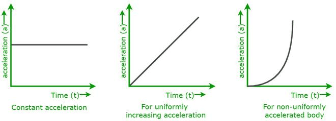
Acceleration vs. Time Graphs:

• Area under curve represents velocity change
• Zero line indicates constant velocity
• Positive values indicate increasing velocity (in positive direction)
• Negative values indicate decreasing velocity (in positive direction)

Linearization Techniques

Complex motion relationships often become clearer through linearization. For example, projectile motion data might not obviously reveal the parabolic relationship y = y₀ + v₀t – ½gt². However, plotting y vs. t² creates a linear relationship that simplifies analysis and parameter extraction.

[EQUATION: y = y₀ – ½gt² + v₀t, rearranged for linearization as y vs. t² analysis]

Linearization skills prove essential for laboratory work and data analysis throughout the AP Physics C curriculum.

Computer-Assisted Data Analysis

Modern physics instruction increasingly incorporates computer tools for data collection and analysis. Spreadsheet programs excel at handling large datasets and performing regression analysis on kinematic data.

When using computer analysis tools:

• Understand the underlying physics principles
• Verify computer results with hand calculations
• Recognize when automated fits may be inappropriate
• Maintain proper significant figures in final results

Practice Problems Section

Multiple Choice Problems

Problem 1: A particle moves along a straight line with position given by x(t) = 2t³ – 3t² + t, where x is in meters and t is in seconds. What is the particle’s acceleration at t = 1 second?

A) 2 m/s² B) 6 m/s² C) 9 m/s² D) 12 m/s² E) 15 m/s²

Solution: v(t) = dx/dt = 6t² – 6t + 1 a(t) = dv/dt = 12t – 6 At t = 1 s: a(1) = 12(1) – 6 = 6 m/s² Answer: B

Problem 2: An object is thrown vertically upward with initial velocity 20 m/s. How long does it take to reach maximum height?

A) 1.0 s B) 2.0 s C) 2.5 s D) 4.0 s E) 4.1 s

Solution: At maximum height, v = 0 Using v = v₀ + at: 0 = 20 + (-9.8)t Solving: t = 20/9.8 = 2.04 ≈ 2.0 s Answer: B

Problem 3: A projectile is launched at 30° above horizontal with initial speed 40 m/s. What is the horizontal component of velocity after 2 seconds?

A) 20 m/s B) 35 m/s C) 40 m/s D) 45 m/s E) The horizontal velocity changes during flight

Solution: Horizontal velocity component remains constant in projectile motion vₓ = v₀ cos 30° = 40 × (√3/2) = 40 × 0.866 = 34.6 ≈ 35 m/s Answer: B

Problem 4: Which of the following represents the correct relationship between position, velocity, and acceleration?

A) a = dx/dt B) v = d²x/dt² C) a = dv/dt D) v = da/dt E) x = dv/dt

Solution: Velocity is the first derivative of position: v = dx/dt Acceleration is the first derivative of velocity: a = dv/dt Therefore, acceleration is the second derivative of position: a = d²x/dt² Answer: C

Problem 5: A ball rolls down a frictionless incline making angle θ with horizontal. Its acceleration down the incline is:

A) g B) g sin θ C) g cos θ D) g tan θ E) g/(sin θ)

Solution: The component of gravitational acceleration parallel to the incline is g sin θ Answer: B

Free Response Problems

Problem FR-1: Motion Analysis (15 minutes)

A particle moves along the x-axis with velocity given by v(t) = 3t² – 12t + 9, where v is in m/s and t is in seconds.

a) Find the particle’s acceleration as a function of time. b) Determine when the particle is at rest. c) Calculate the particle’s displacement between t = 0 and t = 4 seconds, assuming x₀ = 0. d) Describe the particle’s motion during the first 4 seconds.

Solution:

a) a(t) = dv/dt = d/dt(3t² – 12t + 9) = 6t – 12 m/s²

b) Particle at rest when v(t) = 0: 3t² – 12t + 9 = 0 Dividing by 3: t² – 4t + 3 = 0 Factoring: (t – 1)(t – 3) = 0 Therefore: t = 1 s and t = 3 s

c) To find displacement, integrate velocity: x(t) = ∫v(t)dt = ∫(3t² – 12t + 9)dt = t³ – 6t² + 9t + C Since x₀ = 0, we have x(0) = 0, so C = 0 Therefore: x(t) = t³ – 6t² + 9t Displacement from t = 0 to t = 4: Δx = x(4) – x(0) = [64 – 96 + 36] – 0 = 4 m

d) Motion description:

• t = 0 to t = 1: v > 0, a < 0 → moving right, slowing down
• t = 1 to t = 3: v < 0, a < 0 (until t = 2), then a > 0 → moving left, speeding up then slowing down
• t = 3 to t = 4: v > 0, a > 0 → moving right, speeding up

Problem FR-2: Projectile Motion (20 minutes)

A cannon fires a projectile from the top of a 100-meter cliff with initial velocity 50 m/s at 37° above horizontal.

a) Calculate the horizontal and vertical components of initial velocity. b) Determine the maximum height above the cliff top reached by the projectile. c) Find the total time of flight until the projectile hits the ground. d) Calculate the horizontal range of the projectile. e) Determine the velocity components when the projectile hits the ground.

Solution:

a) Initial velocity components: v₀ₓ = v₀ cos 37° = 50 × 0.8 = 40 m/s v₀ᵧ = v₀ sin 37° = 50 × 0.6 = 30 m/s

b) Maximum height above cliff: At max height, vᵧ = 0 Using vᵧ² = v₀ᵧ² – 2gh: 0 = 30² – 2(9.8)h Solving: h = 900/(19.6) = 45.9 m

c) Total time of flight: Using y = y₀ + v₀ᵧt – ½gt² with final position y = -100 m (ground level): -100 = 0 + 30t – 4.9t² Rearranging: 4.9t² – 30t – 100 = 0

Using quadratic formula: t = [30 ± √(900 + 1960)]/9.8 = [30 ± 53.5]/9.8 Taking positive root: t = 83.5/9.8 = 8.52 s

d) Horizontal range: R = v₀ₓ × t = 40 × 8.52 = 341 m

e) Velocity components at impact: vₓ = v₀ₓ = 40 m/s (unchanged) vᵧ = v₀ᵧ – gt = 30 – 9.8(8.52) = 30 – 83.5 = -53.5 m/s Final speed = √(40² + 53.5²) = √4460 = 66.8 m/s

Problem FR-3: Experimental Design (15 minutes)

Design an experiment to determine the acceleration due to gravity using a ball dropped from various heights.

a) Describe your experimental setup and procedure. b) Identify the variables you will measure and control. c) Explain how you will analyze your data to find g. d) Discuss potential sources of error and how to minimize them.

Solution:

a) Experimental setup:

• Use a photogate timer system or video analysis
• Drop ball from measured heights (1m, 1.5m, 2m, 2.5m, 3m)
• Release ball from rest to ensure v₀ = 0
• Measure time of fall for each height
• Repeat each measurement multiple times for statistical analysis

b) Variables: Controlled: Initial velocity (zero), ball mass and size, release technique Measured: Drop height (h), fall time (t) Calculated: Acceleration (g)

c) Data analysis: Using h = ½gt² Rearranging: g = 2h/t² Plot h vs. t² → slope = g/2, so g = 2 × slope Alternative: Calculate g for each trial, then find average

d) Error sources and mitigation:

• Air resistance: Use dense, compact ball; limit drop height
• Timing errors: Use electronic timing systems; multiple trials
• Height measurement: Use precise measuring tools; mark drop points
• Release technique: Practice consistent release method; use release mechanism
• Data analysis: Perform uncertainty analysis; check for outliers

Advanced Problem-Solving Scenarios

Problem AS-1: Variable Acceleration

A particle starts from rest and experiences acceleration a(t) = 4 – 2t m/s² for t ≥ 0.

a) Find expressions for velocity and position as functions of time. b) Determine when the particle momentarily stops. c) Calculate the maximum displacement from the starting point. d) Describe the long-term behavior of this motion.

Solution:

a) Finding velocity and position: v(t) = ∫a(t)dt = ∫(4 – 2t)dt = 4t – t² + C₁ Since v(0) = 0: C₁ = 0 Therefore: v(t) = 4t – t²

x(t) = ∫v(t)dt = ∫(4t – t²)dt = 2t² – t³/3 + C₂ Since x(0) = 0: C₂ = 0 Therefore: x(t) = 2t² – t³/3

b) Particle stops when v(t) = 0: 4t – t² = 0 t(4 – t) = 0 Solutions: t = 0 (initial) and t = 4 s

c) Maximum displacement occurs at t = 4 s: x(4) = 2(16) – 64/3 = 32 – 21.33 = 10.67 m

d) Long-term behavior: For t > 4, velocity becomes increasingly negative Acceleration becomes increasingly negative Particle moves in negative direction with increasing speed Position eventually becomes negative (returns through starting point)

Exam Preparation Strategies

Understanding AP Physics C Exam Format

The AP Physics C: Mechanics exam consists of two main sections that test different aspects of your kinematic knowledge:

Multiple Choice Section (45 minutes, 35 questions):

• Emphasizes conceptual understanding and quick problem-solving
• Often includes graphical analysis and interpretation
• Tests ability to select appropriate equations and approaches
• Requires strong grasp of mathematical relationships

Free Response Section (45 minutes, 3 questions):

• Demands detailed problem-solving with full explanations
• Often combines multiple physics concepts
• Requires experimental design and analysis skills
• Tests calculus applications and mathematical rigor

Key Strategies for Kinematic Success

Master the Mathematical Relationships: Memorizing equations isn’t enough – understand how they connect through calculus. Practice taking derivatives and integrals of kinematic functions until these operations become automatic.

Develop Graphical Intuition: Spend significant time analyzing motion graphs. Practice sketching position, velocity, and acceleration graphs for the same motion. This skill appears frequently and builds conceptual understanding.

Practice Systematic Problem-Solving: Use consistent approaches like the GUESS method for all problems. This prevents errors and builds confidence during time pressure.

Connect to Real-World Applications: Understanding how kinematics applies to technology, sports, and engineering helps retention and provides context for abstract concepts.

Common Exam Mistakes and Prevention

Sign Convention Errors: Establish coordinate systems clearly and maintain consistency throughout problems. Draw diagrams showing positive directions.

Calculus Application Mistakes: Remember that derivatives give rates of change while integrals accumulate quantities over time. Practice both operations regularly.

Vector Component Confusion: Always break vectors into components systematically. Use consistent notation and verify that component magnitudes make sense.

Unit Analysis Neglect: Perform dimensional analysis throughout calculations. Units provide valuable error-checking opportunities.

Historical Context: Giants of Kinematics

Understanding the historical development of kinematic concepts enriches your appreciation of these fundamental principles and often provides memorable context for exam preparation.

Galileo Galilei (1564-1642) revolutionized motion analysis by emphasizing mathematical description over philosophical speculation. His inclined plane experiments demonstrated that acceleration could be constant, leading to the kinematic relationships you use today. Galileo’s insight that projectile motion combines horizontal and vertical components independently remains central to modern physics.

Sir Isaac Newton (1642-1727) connected kinematics to dynamics through his laws of motion, showing that kinematic descriptions have underlying physical causes. Newton’s development of calculus provided the mathematical tools necessary for analyzing variable acceleration scenarios.

The mathematical formalism you’ve mastered represents centuries of intellectual development, connecting your studies to the greatest minds in scientific history.

Conclusion and Next Steps: Building Your Physics Foundation

Mastering AP Physics C: Mechanics Unit 1 requires more than memorizing equations – you must develop intuition for how mathematical relationships describe physical reality. The calculus-based approach distinguishes this course from simpler treatments, providing tools for analyzing complex real-world scenarios.

Your kinematic foundation directly supports upcoming units in the AP Physics C curriculum. Forces and Newton’s laws build on your understanding of acceleration. Energy concepts connect to kinematic relationships through work-energy theorems. Momentum principles rely on velocity and impulse relationships. Oscillations and rotation extend kinematic principles to new coordinate systems and motion types.

Recommended Study Strategies

Daily Practice: Solve at least one kinematic problem daily, varying problem types to maintain skill diversity. Focus on areas where you feel less confident.

Concept Mapping: Create visual representations connecting position, velocity, and acceleration through calculus operations. Include graphical relationships and real-world examples.

Group Study: Explain concepts to classmates – teaching others reveals gaps in your understanding and reinforces learning.

Laboratory Extensions: Seek opportunities to collect and analyze real motion data. Understanding experimental aspects enhances theoretical knowledge.

Preparing for Advanced Physics

The analytical skills you’ve developed studying kinematics transfer to advanced physics courses and engineering applications. University physics builds directly on AP Physics C foundations, while engineering disciplines apply kinematic principles to design problems ranging from spacecraft trajectories to manufacturing automation.

Consider exploring connections between kinematics and other scientific disciplines. Biology uses kinematic analysis to study animal locomotion and molecular motion. Chemistry applies motion principles to reaction kinetics and diffusion processes. Earth science uses projectile motion concepts to understand ballistic processes and orbital mechanics.

Your journey through AP Physics C: Mechanics Unit 1 represents the beginning of a deeper understanding of how mathematics describes natural phenomena. The problem-solving strategies, analytical thinking skills, and mathematical sophistication you’ve developed provide tools for tackling complex challenges throughout your scientific career.

Remember that physics mastery comes through persistent practice and conceptual reflection. Continue building on this kinematic foundation as you progress through the AP Physics C curriculum, and maintain connections between mathematical formalism and physical intuition. Success in physics – both on the AP exam and in future studies – depends on this balance between computational skill and conceptual understanding.

The elegant mathematical relationships governing motion that you’ve mastered connect to fundamental principles throughout physics. Whether you pursue engineering, research science, or simply seek to understand the world around you, these kinematic principles provide essential analytical tools for describing and predicting how objects move through space and time.

Recommended –

• The Medical Dream Blueprint: Transforming Academic Weakness into NEET Success – A Zero-to-Hero Journey
• AP Physics 1 Unit 1: Kinematics – The Complete Student Guide to Motion (2025)