Breathing Trouble: Mastering AP Environmental Science Unit 7 – Atmospheric Pollution

The Air We Breathe

Picture this: You wake up in Beijing on a particularly smoggy day, and the air is so thick with pollution that you can barely see the building across the street. The air quality index reads “hazardous,” and millions of people are advised to stay indoors. Now imagine that same scenario playing out in cities across the globe – from Los Angeles to Mexico City, from New Delhi to London. This isn’t science fiction; it’s the reality of atmospheric pollution in our modern world.

Welcome to one of the most pressing environmental challenges of our time, and one of the most important units in your AP Environmental Science curriculum. Unit 7: Atmospheric Pollution isn’t just about memorizing types of pollutants (though you’ll definitely need to know those for the exam). It’s about understanding how human activities have fundamentally altered the composition of our atmosphere and what that means for every living thing on Earth.

Think about it – every breath you take right now contains molecules that have been cycling through our atmosphere for potentially millions of years. But increasingly, those molecules include substances that weren’t there before the Industrial Revolution. Understanding atmospheric pollution means understanding how we’ve changed the very air that sustains life on our planet.

In this comprehensive guide, we’ll explore everything from the chemistry of smog formation to the global implications of acid rain, all while keeping your AP Environmental Science exam success in mind. You’ll discover why some cities have air you can practically chew, learn about the invisible pollutants that might be affecting your health right now, and understand the complex relationships between atmospheric pollution and climate change.

Did You Know? The Great Smog of London in 1952 was so severe that it killed an estimated 4,000 people in just four days and led to the world’s first major air pollution legislation. This event helped launch the modern environmental movement and directly influenced the environmental science curriculum you’re studying today.

By the end of this unit, you’ll not only be prepared to tackle any atmospheric pollution question on the AP Environmental Science exam, but you’ll also have a deeper appreciation for the delicate balance of our atmosphere and why protecting air quality is crucial for our survival.

Fundamental Concepts: The Science Behind the Smog

Understanding Our Atmosphere’s Structure

Before we dive into pollution, let’s establish the foundation. Our atmosphere isn’t just one big blob of air – it’s a carefully layered system, and understanding these layers is crucial for grasping how pollution behaves and affects us.

The troposphere is where we live and breathe, extending from Earth’s surface up to about 10-15 kilometers. This is where virtually all weather occurs and where most atmospheric pollution has its immediate effects. Here’s the key point for your AP exam: temperature generally decreases with altitude in the troposphere, which is why mountains are colder than valleys.

Above that sits the stratosphere (15-50 km), home to the ozone layer that protects us from harmful UV radiation. Temperature actually increases with altitude here due to ozone absorbing UV energy. This temperature inversion is crucial because it prevents most tropospheric air from mixing upward – essentially trapping pollution in the layer where we live.

Study Tip: Remember the troposphere/stratosphere boundary with this memory device: “Tropo-SPHERE is where we live and breathe on our SPHERE (Earth), Strato-SPHERE is where the ozone protects our SPHERE.”

The Chemistry of Clean Air vs. Polluted Air

Clean, dry air is remarkably simple: about 78% nitrogen (N₂), 21% oxygen (O₂), 0.93% argon, and 0.04% carbon dioxide (CO₂). That’s it for the major components. But atmospheric pollution introduces hundreds of additional substances, and understanding their sources, behavior, and effects is the heart of this unit.

Primary pollutants are emitted directly from sources. Think of the black smoke coming from a coal plant’s smokestack – that’s primary pollution. Secondary pollutants form in the atmosphere through chemical reactions. The brownish haze over Los Angeles isn’t directly emitted by cars; it forms when sunlight triggers reactions between primary pollutants.

Major Categories of Atmospheric Pollutants

Let’s break down the big players in atmospheric pollution – the ones you absolutely must know for the AP exam:

Carbon Monoxide (CO) is the silent killer. This colorless, odorless gas forms when carbon-containing fuels burn incompletely. Your car produces it, your gas stove can produce it, and even your fireplace produces it. CO binds to hemoglobin more readily than oxygen does, essentially suffocating you at the cellular level. This is why carbon monoxide detectors save lives.

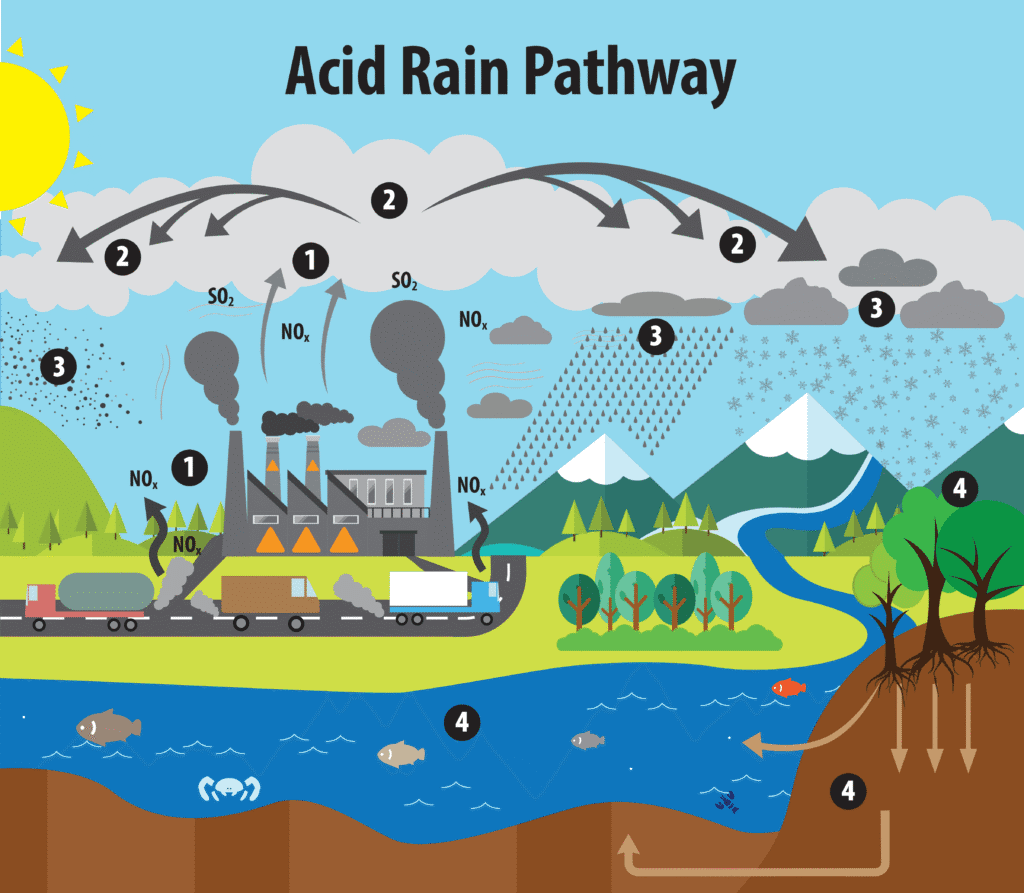
Sulfur Dioxide (SO₂) is the acid rain culprit. Primarily from burning coal and oil that contain sulfur compounds, SO₂ can travel hundreds of miles in the atmosphere. When it combines with water vapor, it forms sulfuric acid – turning rain into a weak acid solution that can damage buildings, forests, and aquatic ecosystems.

Nitrogen Oxides (NOₓ) – notice the “x” because there are several forms – primarily come from high-temperature combustion in vehicles and power plants. The extreme heat causes atmospheric nitrogen and oxygen to combine in ways they normally wouldn’t. These compounds are key players in both acid rain and photochemical smog formation.

Particulate Matter (PM) is probably affecting your health right now, even if you can’t see it. PM₁₀ refers to particles smaller than 10 micrometers (about 1/7th the width of a human hair), while PM₂.₅ particles are even tinier. These microscopic particles can penetrate deep into your lungs and even enter your bloodstream.

Volatile Organic Compounds (VOCs) include everything from the gasoline fumes you smell at gas stations to the solvents in paint and cleaning products. In sunlight, VOCs react with NOₓ to form ground-level ozone – not the good ozone in the stratosphere, but the lung-irritating kind in smog.

The Photochemical Smog Process

Here’s where chemistry meets environmental science in a big way. Photochemical smog formation is a complex process that you need to understand both conceptually and mechanistically for the AP exam.

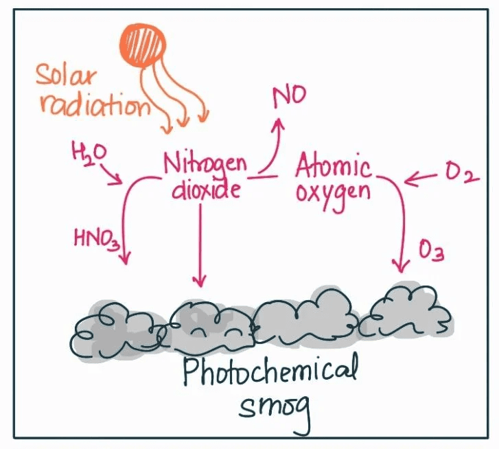
It starts on a sunny morning in a city like Los Angeles. Cars begin their morning commute, emitting NOₓ and VOCs. As sunlight intensifies, it provides the energy needed to break apart NO₂ molecules, creating highly reactive oxygen atoms. These atoms quickly combine with O₂ to form ozone (O₃).

Key Reaction Sequence:

1. NO₂ + sunlight → NO + O
2. O + O₂ → O₃ (ozone)
3. VOCs + NOₓ + sunlight → various secondary pollutants + more O₃

The result? That characteristic brown haze that peaks in the afternoon when sunlight is most intense. This is why ozone alerts typically occur during hot, sunny summer days.

Temperature Inversions: Nature’s Pollution Trap

Understanding temperature inversions is crucial for explaining why pollution sometimes reaches dangerous levels. Normally, air temperature decreases with altitude, allowing warm air near the surface to rise and disperse pollutants. But during an inversion, a layer of warm air sits on top of cooler surface air, creating a “lid” that traps pollutants near the ground.

Los Angeles is famous for inversions because its geography – mountains surrounding a basin – combined with weather patterns creates perfect conditions for trapping smog. Mexico City, Denver, and Salt Lake City face similar challenges.

Did You Know? The word “smog” was coined in London in 1905, combining “smoke” and “fog.” However, London’s smog was primarily sulfur-based from coal burning, while modern cities like Los Angeles deal with photochemical smog from vehicle emissions.

Indoor Air Pollution: The Hidden Threat

While we often focus on outdoor air quality, indoor air pollution can be 2-5 times worse than outdoor air, according to the EPA. This is especially important in developing countries where cooking and heating with biomass fuels inside homes creates dangerous levels of particulate matter and carbon monoxide.

Major indoor pollutants include:

• Radon: A radioactive gas from natural uranium decay in soil and rocks
• Asbestos: From building materials in older structures
• Formaldehyde: From furniture, carpets, and building materials
• Biological pollutants: Mold, dust mites, pet dander
• Combustion byproducts: From gas stoves, fireplaces, and tobacco smoke

The health implications are staggering – the World Health Organization estimates that indoor air pollution causes more deaths annually than outdoor air pollution.

Real-World Applications: Pollution in Action

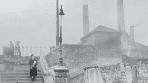
Case Study 1: The Great London Smog of 1952

Let’s travel back to December 1952 in London. A perfect storm of meteorological and human factors created one of the deadliest air pollution events in recorded history, and it fundamentally changed how we think about air quality regulation.

London had been burning coal for centuries, but post-World War II economic pressures meant people were burning lower-quality, high-sulfur coal. When a massive high-pressure system settled over the city, it created a temperature inversion that acted like a giant lid, trapping all the sulfur dioxide, particulate matter, and other pollutants near the ground.

For five days, visibility dropped to less than a meter in some areas. Buses couldn’t run because drivers couldn’t see the road. Concerts were cancelled because audiences couldn’t see the stage. But the real tragedy was human – an estimated 4,000 people died during those five days, with thousands more dying from pollution-related illnesses in the following weeks.

This disaster led directly to the Clean Air Act of 1956, one of the world’s first major pieces of environmental legislation. It established smoke control areas and began the transition away from coal burning in urban areas. The lesson for AP Environmental Science students? Environmental disasters often catalyze policy changes that prevent future tragedies.

Case Study 2: Beijing’s Battle with Air Pollution

Fast-forward to modern-day Beijing, where rapid industrialization and urbanization have created air pollution challenges that make London’s historic smog look mild. Beijing’s pollution is a complex mix of particulate matter from coal burning, vehicle emissions, construction dust, and industrial processes.

During the 2008 Olympics, the Chinese government implemented dramatic measures to improve air quality: they shut down factories, restricted vehicle use, and even used cloud seeding to encourage rain that would wash pollutants out of the air. Air quality improved dramatically, but only temporarily.

The real breakthrough came with China’s “War on Pollution” declared in 2014. Massive investments in renewable energy, stricter emission standards, and the closure of coal-fired power plants have led to significant improvements. Beijing’s PM₂.₅ levels dropped by more than 35% between 2013 and 2018.

Key AP Environmental Science Connection: This case study illustrates how environmental problems often require both technological solutions (cleaner energy sources) and policy interventions (emission standards, economic incentives) working together.

Case Study 3: Mexico City’s High-Altitude Challenge

Mexico City presents a unique case study because its high altitude (2,240 meters above sea level) creates special challenges for air pollution. At high altitudes, there’s less oxygen in the air, so car engines don’t burn fuel as completely, producing more carbon monoxide and other pollutants.

The city’s location in a valley surrounded by mountains creates a natural bowl that traps pollutants, similar to Los Angeles. Temperature inversions are common, especially during winter months when thermal inversions can persist for days.

Mexico City’s approach has been multifaceted:

• Hoy No Circula (No Drive Today) program restricts vehicle use based on license plate numbers
• Conversion of public buses to cleaner-burning compressed natural gas
• Industrial emission controls and fuel quality improvements
• Expansion of the metro system to reduce car dependence

The results have been impressive – despite population growth, air quality has steadily improved since the 1990s. This demonstrates that cities can grow economically while improving environmental quality with the right policies and technologies.

The Acid Rain Story: From Problem to Recovery

Acid rain provides one of environmental science’s great success stories, and it’s a perfect example of how understanding atmospheric chemistry leads to effective policy solutions.

In the 1970s and 1980s, forests in the northeastern United States and southeastern Canada were dying. Lakes were becoming so acidic that fish populations collapsed. The Statue of Liberty’s copper surface was corroding at an alarming rate. The culprit? Sulfur dioxide emissions from coal-fired power plants in the Midwest that were being transported hundreds of miles by prevailing winds.

The Chemistry Behind Acid Rain:

1. SO₂ and NOₓ are released into the atmosphere
2. These gases react with water, oxygen, and other chemicals to form sulfuric and nitric acids
3. These acids fall to Earth as acid rain, snow, or fog
4. Normal rainwater has a pH of about 5.6 (slightly acidic due to dissolved CO₂)
5. Acid rain typically has a pH between 4.2 and 4.4, but can be as low as 2.0

The solution came through the 1990 Clean Air Act Amendments, which created the first large-scale cap-and-trade program for pollution control. Power plants were given emission allowances for SO₂, and they could buy and sell these allowances, creating economic incentives to reduce emissions cost-effectively.

The results exceeded all expectations. SO₂ emissions dropped by more than 70% between 1990 and 2010, while the economy continued to grow. Many lakes and forests have recovered, and the program became a model for other environmental markets, including carbon trading systems.

Global Patterns: Why Some Cities Struggle More

Air pollution isn’t randomly distributed across the globe. Several factors determine why some cities face severe pollution challenges while others maintain relatively clean air:

Geographic factors play a huge role. Cities in valleys (Los Angeles, Mexico City, Salt Lake City) or surrounded by mountains face natural barriers to air circulation. Coastal cities often benefit from sea breezes that help disperse pollutants.

Climate patterns matter enormously. Cities with frequent temperature inversions, low wind speeds, or long periods without rain face greater pollution challenges. This is why Delhi’s pollution peaks during winter months when weather patterns trap pollutants near the surface.

Economic development stage strongly correlates with pollution patterns. The Environmental Kuznets Curve suggests that pollution initially increases with economic development but then decreases as countries become wealthy enough to prioritize environmental quality and can afford cleaner technologies.

Energy sources fundamentally determine a city’s pollution profile. Cities heavily dependent on coal for electricity and heating (like many in China and Eastern Europe) face different challenges than cities powered primarily by natural gas or renewable energy.

Environmental Connections: The Web of Atmospheric Interactions

Atmospheric Pollution and Climate Change: Two Sides of the Same Coin

Here’s a crucial connection for your AP Environmental Science exam: atmospheric pollution and climate change aren’t separate problems – they’re intimately connected processes that often share the same sources and solutions.

Fossil fuel combustion is the primary source of both air pollutants and greenhouse gases. When you burn coal in a power plant, you simultaneously release SO₂ (causing acid rain), NOₓ (contributing to smog), PM (affecting human health), and CO₂ (driving climate change). This means that many solutions to air pollution also help address climate change.

However, the relationship isn’t always straightforward. Some air pollutants actually have cooling effects on the atmosphere. Sulfate aerosols (tiny particles containing sulfur) reflect sunlight back to space, partially offsetting warming from greenhouse gases. This has led to what scientists call the “global dimming” effect – air pollution has actually been masking some of the warming that would otherwise have occurred.

Black carbon (soot) presents a particularly complex case. When it’s suspended in the atmosphere, it absorbs sunlight and contributes to warming. But when it settles on snow and ice, it darkens these surfaces, reducing their ability to reflect sunlight and accelerating melting. This is a major concern in the Arctic, where black carbon from fires and fossil fuel combustion is contributing to rapid ice loss.

Study Tip: For the AP exam, remember that atmospheric pollutants can have both direct health effects (what they do to your lungs) and indirect climate effects (what they do to Earth’s energy balance). Many pollutants have both types of impacts.

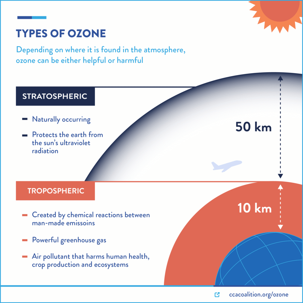
The Ozone Paradox: Good Up High, Bad Nearby

This is one of the most commonly misunderstood concepts in atmospheric science, and it’s frequently tested on the AP Environmental Science exam. Ozone (O₃) is simultaneously our protector and our enemy, depending entirely on where it’s located.

Stratospheric ozone (the “good” ozone) forms naturally when UV radiation breaks apart O₂ molecules, and the resulting oxygen atoms combine with other O₂ molecules. This ozone layer absorbs most of the sun’s harmful UV-B radiation, protecting us from skin cancer, cataracts, and immune system damage.

Tropospheric ozone (the “bad” ozone) forms through photochemical reactions involving pollutants. It’s a major component of smog and can cause respiratory problems, aggravate asthma, and damage crops. Ground-level ozone concentrations typically peak on hot, sunny summer afternoons when photochemical reactions are most active.

Here’s the paradox: we need more ozone in the stratosphere to protect us from UV radiation, but we need less ozone in the troposphere to protect our health. And here’s the kicker – the chemicals that destroy stratospheric ozone (like CFCs) don’t significantly affect tropospheric ozone, while the pollutants that create tropospheric ozone don’t reach the stratosphere in significant quantities.

Air Pollution’s Impact on Ecosystems

Atmospheric pollution doesn’t just affect human health – it profoundly impacts entire ecosystems in ways that cascade through food webs and biogeochemical cycles.

Forest ecosystems face multiple stressors from air pollution. Acid rain leaches essential nutrients like calcium and magnesium from soil while mobilizing toxic aluminum. This nutrient imbalance weakens trees, making them more susceptible to diseases, insects, and weather stress. In the Appalachian Mountains, sugar maples have shown significant decline due to acid rain effects on soil chemistry.

Ozone directly damages plant tissues, causing visible leaf damage and reducing photosynthesis. Crops like soybeans, cotton, and wheat show reduced yields when exposed to elevated ozone levels. This represents a direct economic impact of air pollution on agriculture.

Aquatic ecosystems suffer when acidic precipitation lowers the pH of lakes and streams. Acid-sensitive species like trout and salmon decline first, but entire food webs can collapse as pH drops below critical thresholds. In the Adirondack Mountains of New York, hundreds of lakes became too acidic to support fish populations during the peak of the acid rain crisis.

Nitrogen deposition from NOₓ pollution acts as an unintended fertilizer, altering plant communities by favoring fast-growing, nitrogen-loving species over slower-growing natives. This process, called eutrophication, can fundamentally change ecosystem structure and reduce biodiversity.

The Global Transport of Air Pollution

Air pollution doesn’t respect political boundaries – it’s a truly global phenomenon. Understanding long-range transport of pollutants is crucial for grasping why air pollution requires international cooperation to solve.

Mercury provides a perfect example. Mercury released from coal-fired power plants in Asia can travel across the Pacific Ocean and be deposited in North American ecosystems. Fish in remote Alaskan lakes contain mercury that originated thousands of miles away. This global mercury cycle means that even countries that have reduced their own mercury emissions continue to face contamination from distant sources.

Dust storms transport both natural particles and pollutants across continents. Saharan dust regularly crosses the Atlantic Ocean, affecting air quality in the Caribbean and southeastern United States. These dust events can trigger respiratory problems in sensitive individuals and reduce visibility over vast areas.

Persistent organic pollutants (POPs) like DDT and PCBs can travel through the atmosphere to remote locations where they were never used. These compounds accumulate in polar regions through a process called the grasshopper effect – they evaporate in warm climates, travel through the atmosphere, and condense in colder regions.

Current Research and Trends: The Cutting Edge of Atmospheric Science

Emerging Pollutants and Health Concerns

The field of atmospheric pollution research is rapidly evolving as scientists discover new pollutants and better understand the health effects of existing ones. These emerging trends are reshaping our understanding of air pollution and driving new regulatory approaches.

Ultrafine particles (smaller than PM₀.₁) are receiving increasing attention because they can penetrate deeper into the lungs and cross into the bloodstream more easily than larger particles. These particles are primarily from combustion sources, especially diesel engines and biomass burning. Research suggests they may be more toxic per unit mass than larger particles.

Secondary organic aerosols (SOAs) form when volatile organic compounds undergo complex atmospheric chemistry. Unlike primary particles that are directly emitted, SOAs form in the atmosphere through reactions involving sunlight, oxidants, and precursor compounds. They can account for a large fraction of fine particle mass in urban areas.

Microplastics in the atmosphere represent a completely new category of pollution that wasn’t even recognized a decade ago. Tiny plastic particles from synthetic textiles, tire wear, and plastic degradation are now found in atmospheric samples from remote locations including mountain peaks and polar regions. The health implications are still being studied, but the global distribution suggests widespread exposure.

Advanced Monitoring Technologies

The way we monitor and understand air pollution is being revolutionized by new technologies that provide unprecedented detail about pollutant sources, transport, and effects.

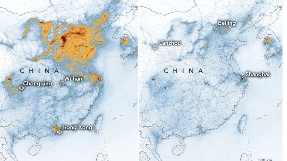
Satellite monitoring now provides daily global maps of various pollutants. NASA’s Aura satellite can track NO₂, SO₂, formaldehyde, and aerosols with spatial resolution fine enough to identify individual power plants and highways. During the COVID-19 lockdowns, satellite data provided dramatic visual evidence of how reduced human activity immediately improved air quality in cities worldwide.

Low-cost sensor networks are democratizing air quality monitoring. Instead of relying on a few expensive government monitoring stations, cities can now deploy hundreds of small, affordable sensors to create detailed pollution maps. This hyperlocal monitoring reveals pollution hotspots and helps communities understand their exposure in unprecedented detail.

Machine learning and artificial intelligence are being applied to predict air quality, identify pollution sources, and understand complex atmospheric chemistry. AI models can now forecast air quality several days in advance with accuracy comparable to weather forecasts, helping people make informed decisions about outdoor activities.

The COVID-19 Air Quality Experiment

The COVID-19 pandemic provided an unprecedented natural experiment in air pollution reduction. When billions of people suddenly stayed home and economic activity plummeted, air quality improved dramatically in cities worldwide. This “anthropause” (human pause) offered valuable insights into pollution sources and the potential for rapid air quality improvements.

In China, NO₂ concentrations dropped by 20-30% during the lockdown period. Los Angeles experienced some of the cleanest air in decades, with smog virtually disappearing from the basin. European cities saw similar improvements, with NO₂ levels dropping by 20-70% in major urban areas.

But the improvements weren’t uniform across all pollutants. While traffic-related pollutants (NO₂, CO) showed dramatic decreases, PM₂.₅ reductions were more modest because particles come from many sources including residential heating, agriculture, and industrial processes that continued during lockdowns.

The pandemic also highlighted the connection between air pollution and respiratory health. Areas with higher long-term PM₂.₅ exposure showed increased COVID-19 mortality rates, suggesting that air pollution may have made populations more vulnerable to the virus.

Wildfire Smoke: A Growing Global Concern

Climate change is increasing the frequency and intensity of wildfires worldwide, creating new air quality challenges that extend far beyond traditional fire-prone regions. Wildfire smoke contains a complex mixture of pollutants including PM₂.₅, carbon monoxide, nitrogen oxides, and numerous toxic organic compounds.

The 2020 wildfire season in the western United States created air quality emergencies across the continent. Smoke from California fires reached as far as Europe, demonstrating the truly global nature of this pollution source. Cities like Portland, Seattle, and San Francisco experienced air quality index values above 300 (hazardous) for days at a time.

Prescribed burning presents a management dilemma. Controlled fires reduce wildfire risk by removing accumulated fuel, but they also create air pollution. Fire managers now use sophisticated atmospheric models to conduct burns when weather conditions will minimize smoke impacts on populated areas.

The Role of Atmospheric Pollution in Environmental Justice

Emerging research reveals that air pollution exposure isn’t equally distributed across populations. Low-income communities and communities of color often face disproportionately high exposure to air pollutants, creating environmental justice concerns that are increasingly being addressed in policy and research.

Redlining and pollution exposure studies show that historically segregated neighborhoods often have higher pollution levels due to their proximity to highways, industrial facilities, and other pollution sources. These patterns persist decades after discriminatory housing policies were eliminated.

Cumulative exposure research examines how multiple environmental stressors (air pollution, noise, toxic waste sites) concentrate in certain communities, creating compounding health risks. This approach moves beyond looking at single pollutants to understand total environmental health burdens.

Community-based monitoring programs are empowering residents to measure their own air quality and advocate for improvements. These citizen science initiatives often reveal pollution hotspots that government monitoring networks miss.

Study Guide Section: Mastering the Material

Essential Formulas and Calculations

While AP Environmental Science isn’t primarily a math-heavy course, there are several key calculations related to atmospheric pollution that you should master:

Air Quality Index (AQI) Calculation:
The AQI converts pollutant concentrations into a standardized scale from 0-500. The basic formula is:
AQI = [(C – C_low)/(C_high – C_low)] × (AQI_high – AQI_low) + AQI_low

Where C is the pollutant concentration, and the other values come from EPA breakpoint tables.

Parts per Million (ppm) and Parts per Billion (ppb) Conversions:

• 1 ppm = 1,000 ppb
• For gases: ppm = (mass of pollutant/mass of air) × 10⁶
• To convert between ppm and μg/m³, you need molecular weight and temperature/pressure

Acid Rain pH Calculations:
Remember that pH is logarithmic:

• Normal rainwater pH ≈ 5.6 (due to dissolved CO₂)
• Acid rain pH typically 4.2-4.4
• Each unit decrease represents a 10× increase in acidity

Study Tip: The AP exam rarely requires complex calculations, but understanding these relationships helps you interpret data and graphs correctly.

Key Concepts Summary

Primary vs. Secondary Pollutants:

• Primary: Directly emitted (CO, SO₂, NOₓ, particulates)
• Secondary: Form through atmospheric reactions (O₃, acid rain, some particulates)

Major Pollutant Sources and Effects:

• Mobile sources: Cars, trucks, planes, ships
• Stationary sources: Power plants, factories, residential heating
• Area sources: Agricultural activities, construction, wildfires
• Natural sources: Volcanoes, dust storms, biological processes

Health Effect Categories:

• Acute effects: Immediate responses (eye irritation, coughing)
• Chronic effects: Long-term exposure results (lung cancer, heart disease)
• Sensitive populations: Children, elderly, people with respiratory conditions

Memory Devices and Study Tips

For remembering criteria pollutants, use “SLONP-CO”:

• Sulfur dioxide (SO₂)
• Lead (Pb)
• Ozone (O₃)
• Nitrogen dioxide (NO₂)
• Particulate matter (PM)
• COrbon monoxide (CO)

For photochemical smog formation: “Night Owl Vehicle Smog”

• NOₓ and VOCs emitted
• Oxygen atoms form from NO₂ + sunlight
• Various reactions create secondary pollutants
• Smog peaks in afternoon

For acid rain formation: “Some Nasty Weather Arrives”

• SO₂ and NOₓ released
• Natural oxidation in atmosphere
• Water combines to form acids
• Acid precipitation falls

Common AP Exam Question Types

Data Interpretation Questions: You’ll often see graphs showing pollutant concentrations over time, AQI values for different cities, or emissions trends. Practice reading axes carefully and identifying patterns, trends, and anomalies.

Cause and Effect Relationships: Be prepared to explain how specific human activities lead to particular types of pollution and environmental effects. For example: “Explain how increased automobile use in developing countries might affect both local air quality and global climate.”

Policy Analysis: Questions often ask you to evaluate the effectiveness of different approaches to pollution control. Understand the strengths and weaknesses of command-and-control regulations versus market-based approaches like cap-and-trade.

Cross-Unit Connections: Atmospheric pollution connects to many other APES units. Be ready to discuss how air pollution relates to human health (Unit 8), energy production (Units 6), and land use (Units 5).

Advanced Exam Strategies

For Free Response Questions (FRQs):

1. Always define terms if the question asks you to discuss a concept
2. Use specific examples from case studies when possible
3. Show relationships between causes and effects clearly
4. Address all parts of multi-part questions
5. Use data from any provided graphs or tables to support your answers

For Multiple Choice:

1. Eliminate obviously wrong answers first
2. Look for qualifiers like “always,” “never,” “most,” “least”
3. Pay attention to units in calculation problems
4. Consider all options before selecting the best answer
5. Don’t overthink – your first instinct is often correct

Time Management Tips:

• Spend about 1 minute per multiple choice question
• For FRQs, budget your time based on point values
• Leave time to review and check your work
• If you’re stuck on a question, mark it and return later

Practice Questions: Test Your Knowledge

Multiple Choice Questions

1. Which of the following is a secondary air pollutant?
   a) Carbon monoxide from vehicle exhaust
   b) Sulfur dioxide from coal combustion
   c) Ground-level ozone from photochemical reactions
   d) Lead particles from gasoline combustion
   e) Particulate matter from industrial smokestacks
2. The formation of photochemical smog requires all of the following EXCEPT:
   a) Nitrogen oxides (NOₓ)
   b) Volatile organic compounds (VOCs)
   c) Sunlight
   d) Sulfur dioxide (SO₂)
   e) Warm temperatures
3. A temperature inversion in the atmosphere:
   a) Always occurs at night
   b) Helps disperse air pollutants
   c) Traps pollutants near Earth’s surface
   d) Only affects mountainous regions
   e) Reduces photochemical smog formation
4. Which of the following best explains why cities in valleys often have worse air quality than coastal cities?
   a) Valleys receive less sunlight for photochemical reactions
   b) Valley cities typically have more industrial activity
   c) Mountains surrounding valleys trap pollutants and limit air circulation
   d) Coastal winds always blow pollution out to sea
   e) Valley cities burn more fossil fuels per capita
5. The pH of normal rainwater is approximately 5.6 due to:
   a) Natural sulfur compounds in the atmosphere
   b) Dissolved carbon dioxide forming weak carbonic acid
   c) Nitrogen oxides from lightning
   d) Sea salt particles in the atmosphere
   e) Natural organic acids from vegetation

Answer Key:

1. c) Ground-level ozone forms through atmospheric reactions between primary pollutants
2. d) SO₂ is not required for photochemical smog formation
3. c) Temperature inversions create a “lid” that traps pollutants
4. c) Geographic barriers limit air circulation and pollutant dispersion
5. b) CO₂ + H₂O → H₂CO₃ (carbonic acid)

Free Response Questions

Question 1: A city experiences frequent episodes of poor air quality during summer months, with ozone levels regularly exceeding health standards on hot, sunny days.

a) Explain the chemical process that leads to ground-level ozone formation, including the role of precursor pollutants and meteorological conditions. (4 points)

b) Describe two specific strategies the city could implement to reduce ozone formation, and explain how each strategy would be effective. (4 points)

c) Discuss why ozone concentrations typically peak in the afternoon rather than during morning rush hour when traffic emissions are highest. (2 points)

Sample Answer Framework:
a) NOₓ and VOCs are emitted from vehicles and industry → Sunlight breaks apart NO₂ molecules → Free oxygen atoms combine with O₂ to form O₃ → Process enhanced by warm temperatures and stagnant air conditions

b) Strategies might include: Reduce vehicle emissions through cleaner fuel standards or electric vehicle incentives → Reduce industrial VOC emissions through better controls → Improve public transportation to reduce vehicle usage → Each explanation should connect the strategy to reducing precursor pollutants

c) Time delay between emissions and peak formation → Chemical reactions require several hours to proceed → Peak sunlight intensity occurs in afternoon → Morning emissions have time to undergo photochemical reactions

Question 2: The graph below shows SO₂ emissions from a region over a 30-year period, with a sharp decline beginning in 1990.

[Imagine a graph showing steady high emissions 1980-1990, then sharp decline 1990-2010]

a) Identify and explain one likely cause of the sharp decline in SO₂ emissions beginning in 1990. (3 points)

b) Describe two environmental benefits that would result from this reduction in SO₂ emissions. (4 points)

c) Explain one reason why SO₂ emissions might not decline to zero even with strict environmental regulations. (3 points)

Sample Answer Framework:
a) Clean Air Act Amendments of 1990 established cap-and-trade program for SO₂ → Created economic incentives for power plants to reduce emissions → Companies could profit by reducing emissions below their allowances

b) Reduced acid rain formation → Less acidification of lakes and forests → Improved human health from reduced particulate matter → Less building and monument damage → Better visibility

c) Some industrial processes inherently produce SO₂ → Natural sources like volcanoes continue → Complete elimination might be economically prohibitive → Some regions may lack access to low-sulfur fuels

Data Analysis Questions

Question 3: The table below shows Air Quality Index (AQI) values for different pollutants in two cities on the same day:

Pollutant	City A	City B
PM₂.₅	95	45
O₃	78	120
NO₂	65	85
SO₂	25	180
CO	55	35

a) Determine which city has worse overall air quality and explain your reasoning. (3 points)

b) Based on the pollutant patterns, suggest the most likely primary source of air pollution in each city. (4 points)

c) Recommend specific health precautions for sensitive individuals in the city with worse air quality. (3 points)

Sample Answer Framework:
a) City B has worse overall air quality → Overall AQI is determined by the highest individual pollutant AQI → City B’s SO₂ AQI of 180 is in the “unhealthy” range → This single pollutant makes City B’s air quality worse overall

b) City A: High PM₂.₅ and moderate other pollutants suggest vehicle emissions and possibly biomass burning → City B: Very high SO₂ suggests coal-fired power plants or heavy industry as primary source → Other pollutants in City B also elevated, consistent with industrial sources

c) For City B (worse air quality): Limit outdoor activities, especially strenuous exercise → People with respiratory conditions should stay indoors → Use air purifiers indoors if available → Wear N95 masks if must go outside → Monitor air quality forecasts

Conclusion and Further Exploration

Congratulations! You’ve just completed a comprehensive journey through AP Environmental Science Unit 7: Atmospheric Pollution. From the chemistry of smog formation to the global transport of mercury, from the Great London Smog to Beijing’s modern air quality challenges, you now have the knowledge and analytical tools to understand one of our most pressing environmental issues.

But your learning doesn’t have to stop here. Atmospheric pollution is a rapidly evolving field with new discoveries, technologies, and policy approaches emerging regularly. The COVID-19 pandemic showed us that rapid improvements in air quality are possible when we dramatically change our behavior. Climate change is altering pollution patterns through increased wildfire activity and changing weather patterns. New monitoring technologies are revealing pollution sources and health effects we never knew existed.

As you prepare for the AP Environmental Science exam, remember that atmospheric pollution concepts connect to virtually every other unit in the course. The fossil fuels that power our energy systems (Unit 6) create the emissions that pollute our air. The cities where most humans now live (Unit 5) concentrate both pollution sources and vulnerable populations. The health effects of air pollution (Unit 8) create enormous economic and social costs. Understanding these connections will serve you well on the exam and in your future environmental studies.

Most importantly, atmospheric pollution isn’t just an academic subject – it’s a real-world challenge that affects every breath you take. The concepts you’ve learned here will help you make informed decisions as a citizen, consumer, and potentially as a future environmental professional.

Additional Resources for Deeper Learning

EPA AirNow Website (airnow.gov): Real-time air quality data and forecasts for your area, plus educational resources about different pollutants and health effects.

NASA’s Global Climate Change and Global Warming (climate.nasa.gov): Satellite data and visualizations showing how air pollution patterns change over time and connect to climate change.

World Health Organization Air Pollution Database: Global air quality data and health impact assessments that put local pollution problems in international context.

State of Global Air Report (Annual publication by Health Effects Institute): Comprehensive analysis of global air pollution trends and health impacts, updated annually with the latest research.

C40 Cities Climate Leadership Group: Case studies of how major cities worldwide are tackling air pollution and climate change simultaneously.

Final Exam Success Tips

Remember that the AP Environmental Science exam rewards depth of understanding over memorization of facts. Focus on understanding processes, relationships, and connections rather than just learning lists of pollutants or regulations. Practice explaining concepts in your own words, and always be ready to provide specific examples from the case studies we’ve discussed.

The atmospheric pollution unit is often one of the most heavily tested on the AP exam because it connects to so many other environmental issues. Your thorough understanding of these concepts will serve you well not just in the pollution-specific questions, but in questions about energy, human health, climate change, and environmental policy throughout the exam.

Good luck with your studies, and remember – every breath you take connects you to the global atmospheric system we’ve explored together. Use that connection to stay motivated in your environmental science journey!

This comprehensive guide represents the culmination of decades of atmospheric science research and environmental policy development. The air quality improvements we’ve seen in many parts of the world prove that with scientific understanding, effective policy, and public commitment, we can solve even our most challenging environmental problems. The future of our atmosphere – and our planet – depends on informed citizens like you.

Recommended –

• AP Environmental Science Unit 5: Land and Water Use – Your Complete Study Guide
• AP Environmental Science Unit 6: Energy Resources and Consumption – Your Complete Study Guide