

Introduction: The Invisible Forces That Power Our World
Every time you reach for a doorknob and feel that sudden shock, or watch your hair stand up when you rub a balloon against it, you’re witnessing the fundamental forces that govern our universe. These aren’t just classroom curiosities-they’re the same principles that power your smartphone, enable MRI machines to peer inside the human body, and allow scientists to manipulate individual atoms.
Electric charges and fields form the foundation of electromagnetism, one of the four fundamental forces in nature. From the neurons firing in your brain as you read this to the GPS satellites orbiting Earth, electromagnetic phenomena shape every aspect of modern life. Understanding these concepts isn’t just about passing an exam-it’s about grasping the invisible architecture that makes our technological world possible.
In this unit, you’ll discover how charged particles create invisible fields that extend throughout space, how these fields interact with other charges, and how a brilliant insight by Carl Friedrich Gauss revolutionized our understanding of electric fields. You’ll learn to think like a physicist, using mathematical tools to predict and explain phenomena that seem almost magical at first glance.
Whether you’re planning a career in engineering, medicine, research, or any field touched by technology, the concepts in this unit will serve as your foundation for understanding how the universe works at its most fundamental level.
Learning Objectives: Your Roadmap to Mastery
By the end of this unit, you’ll be able to:
Conceptual Understanding:
- Explain the nature of electric charge and the fundamental principles governing charged particles
- Describe how electric fields are created by charge distributions and how they affect other charges
- Apply conservation of charge in various physical situations
- Understand the relationship between electric fields and electric potential
Mathematical Skills:
- Calculate electric forces using Coulomb’s Law in one and multiple dimensions
- Determine electric field strength and direction for point charges and continuous charge distributions
- Apply Gauss’s Law to solve complex electrostatics problems
- Analyze the motion of charged particles in uniform electric fields
Laboratory Applications:
- Design experiments to investigate electrostatic phenomena
- Analyze data from electric field mapping experiments
- Understand the principles behind common electrostatic devices
Problem-Solving Mastery:
- Tackle multi-step problems involving combinations of charges, fields, and forces
- Apply superposition principles to complex charge configurations
- Use symmetry arguments to simplify challenging problems
Section 1: The Foundation – Understanding Electric Charge
What Makes Something “Charged”?
Imagine you could zoom in on any object around you-your pencil, your desk, even your own hand-until you could see individual atoms. What you’d discover is that everything is made of particles that carry fundamental electric charges. Protons carry positive charge, electrons carry negative charge, and neutrons are electrically neutral.
But here’s what makes this fascinating: in most objects, the number of protons and electrons is exactly equal, making the object electrically neutral overall. It’s only when this delicate balance is disrupted that we observe the phenomena we call “static electricity.”
Real-World Physics: When you shuffle across a carpet in dry weather, you’re literally stealing electrons from the carpet fibers and depositing them on your body. This creates an imbalance-you become negatively charged while the carpet becomes positively charged. The “shock” you feel when touching a doorknob is electrons jumping back to restore electrical balance.
The Fundamental Properties of Electric Charge
Electric charge exhibits several crucial properties that form the foundation of all electromagnetic phenomena:
Conservation of Charge: In any isolated system, the total electric charge remains constant. Charges can be transferred from one object to another, but they cannot be created or destroyed. This principle, discovered through careful experimentation, is one of the most fundamental laws in physics.
Quantization of Charge: All electric charges in nature come in discrete multiples of the elementary charge (e = 1.602 × 10^-19 coulombs). You can’t have 1.5 electrons worth of charge-it’s always whole numbers.
Superposition: The total effect of multiple charges is simply the sum of their individual effects. This seemingly simple principle becomes incredibly powerful when dealing with complex charge distributions.
Types of Charging Processes
Understanding how objects become charged is crucial for both conceptual understanding and practical applications:
Friction (Triboelectric Effect): When two different materials are rubbed together, electrons transfer from one to the other based on their relative positions in the triboelectric series. This is why rubber combs attract paper after being rubbed with wool.
Conduction: When a charged object touches a conductor, charges redistribute to reach equilibrium. This is why touching a metal doorknob after walking across carpet neutralizes your charge.
Induction: Even without direct contact, nearby charges can cause redistribution of charge in conductors. This principle is used in electrostatic generators and lightning rods.
Physics Check: Can you explain why your hair is attracted to a charged balloon even though your hair starts electrically neutral? Think about what happens to the charges in your hair when the balloon approaches.
Section 2: Coulomb’s Law – The Mathematics of Electric Force
The Discovery That Changed Everything
In 1785, Charles-Augustin de Coulomb used an ingenious torsion balance to measure the forces between charged objects. His discovery revealed that electric forces follow a remarkably simple mathematical relationship-one that mirrors Newton’s law of universal gravitation but with a crucial difference in sign behavior.
[EQUATION: Coulomb’s Law: F = k(q₁q₂)/r² where k = 8.99 × 10⁹ N⋅m²/C², q₁ and q₂ are the charges in coulombs, r is the distance between charges in meters, and F is the force in newtons]
Understanding the Inverse Square Relationship
The r² term in the denominator isn’t just mathematical convenience-it reflects something profound about how effects spread through three-dimensional space. As you move twice as far from a charge, the force becomes four times weaker. This same relationship appears throughout physics, from gravity to light intensity, because it describes how influences propagate through our three-dimensional universe.
Common Error Alert: Students often forget that Coulomb’s Law gives the magnitude of force. The direction must be determined separately using the principle that like charges repel and opposite charges attract.
Vector Nature of Electric Forces
Electric forces are vectors, which means they have both magnitude and direction. When dealing with multiple charges, you must use vector addition to find the net force:
Problem-Solving Strategy:
- Calculate the magnitude of each individual force using Coulomb’s Law
- Determine the direction of each force based on charge signs
- Break forces into x and y components
- Add components separately
- Use Pythagorean theorem to find magnitude of net force
- Use trigonometry to find direction
Worked Example: Three Charges in a Line
Let’s solve a classic AP Physics C problem: Three charges are arranged along a straight line. q₁ = +2.0 μC is at the origin, q₂ = -3.0 μC is at x = 4.0 cm, and q₃ = +1.0 μC is at x = 6.0 cm. Find the net force on q₃.
Step 1: Identify given information
- q₁ = +2.0 × 10⁻⁶ C at x = 0
- q₂ = -3.0 × 10⁻⁶ C at x = 0.04 m
- q₃ = +1.0 × 10⁻⁶ C at x = 0.06 m
Step 2: Calculate force from q₁ on q₃
- Distance: r₁₃ = 0.06 m
- F₁₃ = (8.99 × 10⁹)(2.0 × 10⁻⁶)(1.0 × 10⁻⁶)/(0.06)² = 5.0 N
- Direction: Since both charges are positive, the force is repulsive (rightward)
Step 3: Calculate force from q₂ on q₃
- Distance: r₂₃ = 0.02 m
- F₂₃ = (8.99 × 10⁹)(3.0 × 10⁻⁶)(1.0 × 10⁻⁶)/(0.02)² = 67.4 N
- Direction: Since charges have opposite signs, the force is attractive (leftward)
Step 4: Find net force
- Net force = -67.4 + 5.0 = -62.4 N (leftward)
This example illustrates a key insight: the closest charge usually dominates the interaction, even if it’s not the largest charge.
Section 3: Electric Fields – Visualizing the Invisible
From Forces to Fields: A Conceptual Revolution
While Coulomb’s Law tells us about forces between charges, it requires us to know where all charges are located. Electric fields provide a more elegant approach: they describe the “influence” that charges create in the space around them, independent of what other charges might be present.
Think of an electric field as an invisible landscape of potential force. Just as a mountain creates a gravitational field that would pull on any mass placed nearby, a charged particle creates an electric field that would push or pull on any charge placed in its vicinity.
[EQUATION: Electric Field: E = F/q where E is electric field strength in N/C, F is the force a test charge would experience in newtons, and q is the magnitude of the test charge in coulombs]
Electric Field Due to Point Charges
For a point charge, we can combine Coulomb’s Law with the definition of electric field:
[EQUATION: Electric Field of Point Charge: E = kq/r² where q is the source charge creating the field, r is the distance from the source charge, and E points radially away from positive charges or toward negative charges]
The Principle of Superposition for Electric Fields
One of the most powerful aspects of electric fields is that they add vectorially. The total electric field at any point is simply the vector sum of the electric fields created by all charges in the system.
Real-World Physics: This superposition principle is what makes modern electronics possible. In a computer processor, millions of electric fields from different components combine to create precisely controlled forces on electrons, allowing for computation at incredible speeds.
Visualizing Electric Fields with Field Lines
Electric field lines provide a visual representation of electric fields that helps us understand complex charge distributions:
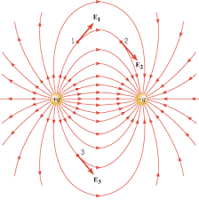
Field Line Rules:
- Lines start on positive charges and end on negative charges
- Line density indicates field strength
- Lines never cross each other
- Lines are tangent to the field direction at every point
Electric Fields of Continuous Charge Distributions
Real-world situations often involve charge distributed over extended objects rather than concentrated at points. For these situations, we use integration to find the electric field:
[EQUATION: Electric Field Integration: E = ∫(kdq/r²) where the integral is taken over the entire charge distribution]
For common geometries, this integration yields elegant results:
Infinite Line of Charge: E = λ/(2πε₀r) where λ is linear charge density
Infinite Plane of Charge: E = σ/(2ε₀) where σ is surface charge density
Problem-Solving Strategy for Continuous Distributions:
- Choose an appropriate coordinate system
- Identify the charge element (dq)
- Express dq in terms of charge density and geometric elements
- Set up the integral for the electric field components
- Use symmetry to simplify when possible
- Evaluate the integral
Section 4: Gauss’s Law – The Elegant Shortcut
The Genius of Carl Friedrich Gauss
In 1835, Carl Friedrich Gauss published a theorem that would revolutionize how physicists approach electric field problems. Gauss’s Law provides an elegant relationship between electric fields and the charges that create them, often allowing us to solve complex problems that would be nearly impossible using direct integration.
[EQUATION: Gauss’s Law: ∮E⋅dA = Q_enclosed/ε₀ where ∮ represents a closed surface integral, E is the electric field, dA is a differential area element, Q_enclosed is the total charge inside the surface, and ε₀ = 8.85 × 10⁻¹² C²/N⋅m² is the permittivity of free space]
Understanding the Gaussian Surface
The key to applying Gauss’s Law effectively is choosing the right Gaussian surface-an imaginary closed surface that we use to evaluate the flux integral. The surface should be chosen to take advantage of the symmetry of the charge distribution.
Common Gaussian Surfaces:
- Spherical: For point charges or spherically symmetric distributions
- Cylindrical: For infinite lines of charge or cylindrical symmetry
- Pillbox (flat cylinder): For infinite planes of charge or planar symmetry
When Gauss’s Law is Most Powerful
Gauss’s Law is particularly useful when the charge distribution has sufficient symmetry that the electric field magnitude is constant over portions of the Gaussian surface and the field is perpendicular to the surface.
High-Symmetry Examples:
- Spherical Symmetry: Point charges, uniformly charged spheres
- Cylindrical Symmetry: Infinite lines of charge, charged cylinders
- Planar Symmetry: Infinite planes of charge, parallel plate capacitors
Worked Example: Electric Field Inside a Conducting Sphere
Consider a solid conducting sphere of radius R carrying total charge Q. Let’s use Gauss’s Law to find the electric field at different locations.
Case 1: Inside the conductor (r < R)
In electrostatic equilibrium, the electric field inside any conductor must be zero. We can prove this using Gauss’s Law:
Choose a spherical Gaussian surface of radius r < R centered at the sphere’s center.
Since E = 0 everywhere inside the conductor:
∮E⋅dA = 0
Therefore: Q_enclosed/ε₀ = 0, which means Q_enclosed = 0
This proves that there can be no net charge anywhere inside a conductor-all charge resides on the surface.
Case 2: Outside the conductor (r > R)
Choose a spherical Gaussian surface of radius r > R. By symmetry, the electric field has constant magnitude and points radially:
∮E⋅dA = E(4πr²) = Q/ε₀
Therefore: E = Q/(4πε₀r²) = kQ/r²
Notice this is identical to the field of a point charge-the spherical conductor looks like a point charge from the outside.
Historical Context: This result explained why Benjamin Franklin’s lightning rod works. The sharp point concentrates electric field, encouraging lightning to strike the rod rather than the building.
Section 5: Electric Potential and Potential Energy
From Force to Energy: A New Perspective
While electric fields tell us about forces, electric potential provides an energy-based approach to electrostatics. Just as gravitational potential energy helps us analyze motion under gravity, electric potential energy allows us to understand the behavior of charges in electric fields.
[EQUATION: Electric Potential Energy: U = qV where U is potential energy in joules, q is the charge in coulombs, and V is electric potential in volts]
[EQUATION: Electric Potential: V = kq/r for a point charge, where V is measured in volts (joules per coulomb)]
The Relationship Between Field and Potential
Electric field and potential are intimately related-the field points in the direction of the greatest decrease in potential:
[EQUATION: Relationship Between E and V: E = -∇V or in one dimension, E = -dV/dx]
This relationship allows us to find electric fields from potential distributions or vice versa, often simplifying complex problems.
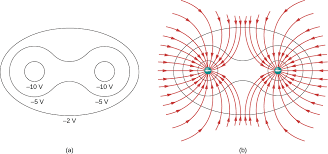
Equipotential Surfaces and Field Lines
Equipotential surfaces are three-dimensional regions where the electric potential has the same value everywhere. These surfaces have a crucial relationship with electric field lines:
- Electric field lines are always perpendicular to equipotential surfaces
- No work is required to move a charge along an equipotential surface
- Field strength is inversely related to the spacing between equipotential surfaces
Applications in Technology
Understanding electric potential is crucial for designing electronic devices:
Real-World Physics: The touchscreen on your phone works by detecting tiny changes in electric potential when your finger (a conductor) approaches the screen. Your finger distorts the electric field pattern, and sophisticated electronics detect these changes to determine where you touched.
Section 6: Motion of Charges in Electric Fields
Charged Particles as Projectiles
When a charged particle enters a uniform electric field, it behaves remarkably similar to a projectile in a gravitational field. The key difference is that the “gravitational” acceleration depends on the charge-to-mass ratio of the particle.
[EQUATION: Acceleration in Electric Field: a = qE/m where a is acceleration, q is particle charge, E is electric field strength, and m is particle mass]
Trajectory Analysis
For a particle with initial velocity v₀ entering a uniform electric field perpendicular to its motion:
Horizontal Motion: x = v₀t (constant velocity)
Vertical Motion: y = ½(qE/m)t² (constant acceleration)
The trajectory is parabolic, just like projectile motion, but the “gravitational” acceleration is qE/m instead of g.
Applications in Modern Technology
This physics forms the foundation of numerous technologies:
Cathode Ray Tubes (CRTs): Electrons are accelerated and deflected by electric fields to create images on phosphorescent screens.
Mass Spectrometry: Different ions follow different curved paths in combined electric and magnetic fields, allowing scientists to determine molecular masses with incredible precision.
Particle Accelerators: Electric fields accelerate charged particles to enormous speeds for fundamental physics research.
Real-World Physics: The Large Hadron Collider uses electric fields to accelerate protons to 99.9999991% the speed of light. At these speeds, the protons have as much kinetic energy as a flying mosquito-concentrated into a space trillions of times smaller!
Section 7: Conductors in Electrostatic Equilibrium
The Special Properties of Conductors
Conductors contain charges that are free to move, leading to unique behaviors in electrostatic situations. Understanding these properties is crucial for applications ranging from lightning protection to electronic device design.
Key Properties of Conductors in Equilibrium:
- Electric field inside is zero
- All excess charge resides on the surface
- Electric field at the surface is perpendicular to the surface
- The entire conductor is at the same electric potential
Charging by Induction
One of the most elegant demonstrations of conductor properties is charging by induction:
- Bring a charged rod near (but not touching) a neutral conductor
- The electric field from the rod pushes mobile charges in the conductor
- One side becomes negatively charged, the other positively charged
- Connect one side to ground to remove charge
- Remove the ground connection, then remove the rod
- The conductor now has a net charge opposite to the original rod
Problem-Solving Strategy for Conductor Problems:
- Identify regions where E = 0 (inside conductors)
- Apply boundary conditions at conductor surfaces
- Use Gauss’s Law with appropriate surfaces
- Remember that conductors are equipotential volumes
Electrostatic Shielding
The zero electric field inside conductors leads to an important application: electrostatic shielding. A conducting enclosure protects its interior from external electric fields.
Real-World Physics: Your car acts as a Faraday cage during lightning storms. Even if lightning strikes the car, the current flows around the outside metal shell, leaving passengers safe inside. This same principle protects sensitive electronics in metal enclosures.
Section 8: Advanced Applications and Problem-Solving Strategies
Combining Multiple Concepts
The most challenging AP Physics C problems require you to integrate concepts from across the unit. These problems test your ability to:
- Apply conservation principles (energy, charge)
- Use symmetry arguments effectively
- Combine field and potential concepts
- Analyze motion in complex field configurations
Systems of Multiple Charges
When dealing with systems containing multiple charges:
- Identify symmetries that can simplify calculations
- Use superposition for both fields and potentials
- Consider energy approaches when forces are complex
- Apply conservation laws to constrain possible solutions
Experimental Design Considerations
When designing electrostatics experiments:
- Control for humidity – moisture affects charge retention
- Use appropriate materials – understand triboelectric series
- Minimize external fields – earth’s field, nearby conductors
- Account for charge leakage – even good insulators have some conductivity
Laboratory Connection: The Millikan oil drop experiment used these principles to measure the charge of individual electrons. By balancing gravitational and electric forces on tiny charged oil droplets, Millikan could determine that charge comes in discrete units.
Practice Problems Section: Mastering the Concepts
Multiple Choice Questions
Problem 1: Two point charges, +2Q and -Q, are separated by distance d. At what point along the line connecting them is the electric field zero?
A) d/4 from the +2Q charge
B) d/3 from the +2Q charge
C) d/2 from the +2Q charge
D) 2d/3 from the +2Q charge
E) The electric field is never zero
Solution: At the point where E = 0, the fields from both charges must be equal in magnitude but opposite in direction. Let x be the distance from +2Q to this point.
From +2Q: E₁ = k(2Q)/x²
From -Q: E₂ = kQ/(d-x)²
Setting E₁ = E₂:
k(2Q)/x² = kQ/(d-x)²
2/x² = 1/(d-x)²
2(d-x)² = x²
2(d² – 2dx + x²) = x²
2d² – 4dx + 2x² = x²
x² – 4dx + 2d² = 0
Using the quadratic formula:
x = (4d ± √(16d² – 8d²))/2 = (4d ± 2√2d)/2 = d(2 ± √2)
Since x must be between 0 and d, we take x = d(2 – √2) ≈ 0.59d
Answer: None of the given options exactly match, but D) 2d/3 ≈ 0.67d is closest.
Problem 2: A uniform electric field E points in the +x direction. A proton is released from rest at the origin. After time t, what is the proton’s kinetic energy?
A) ½(eE)²t²/m
B) (eE)²t²/(2m)
C) eEt²/(2m)
D) ½eEt
E) eEt
Solution:
The force on the proton: F = eE
Acceleration: a = F/m = eE/m
Velocity after time t: v = at = (eE/m)t
Kinetic energy: KE = ½mv² = ½m(eE/m)²t² = (eE)²t²/(2m)
Answer: B
Free Response Problems
Problem 3: A thin, uniformly charged rod of length L carries total charge Q. Find the electric field at a point P located at distance R from one end of the rod, along the rod’s perpendicular bisector.
Solution:
Step 1: Set up coordinate system
Place the rod along the x-axis, centered at the origin. Point P is at (0, R).
Step 2: Express charge element
Linear charge density: λ = Q/L
Charge element: dq = λdx = (Q/L)dx
Step 3: Set up field components
For a charge element at position x:
- Distance to P: r = √(x² + R²)
- Field magnitude: dE = k(dq)/r² = k(Q/L)dx/(x² + R²)
Step 4: Resolve components
By symmetry, x-components cancel. Only y-component remains:
dEᵧ = dE cos θ = dE(R/r) = kQ R dx/[L(x² + R²)^(3/2)]
Step 5: Integrate
E = ∫₍₋ₗ/₂₎^⁽ᴸ/²⁾ kQR dx/[L(x² + R²)^(3/2)]
Using substitution or integral tables:
E = kQR/L × [x/(R²√(x² + R²))]₍₋ₗ/₂₎^⁽ᴸ/²⁾
E = kQR/L × [L/2/(R²√(L²/4 + R²)) – (-L/2)/(R²√(L²/4 + R²))]
E = kQL/(LR²√(L²/4 + R²)) = kQ/(R²√(L²/4 + R²))
Step 6: Check limits
- As L → 0: E → 0 (no charge)
- As L → ∞: E → 2kQ/(LR) (infinite line)
- As R → 0: E → ∞ (expected for finite charge)
Problem 4: Two identical conducting spheres, each of radius R, carry charges +3Q and -Q respectively. They are brought into contact briefly, then separated to a large distance d >> R. Find the force between them after separation.
Solution:
Step 1: Apply charge conservation
Total charge before contact = +3Q + (-Q) = +2Q
After contact, charge distributes equally: each sphere has +Q
Step 2: Apply Coulomb’s Law
Since d >> R, treat as point charges:
F = k(Q)(Q)/d² = kQ²/d²
The force is repulsive since both spheres are now positively charged.
Step 3: Verify using energy considerations
Initial potential energy: U₍ᵢ₎ = k(3Q)(-Q)/d = -3kQ²/d
Final potential energy: U₍f₎ = k(Q)(Q)/d = kQ²/d
The change in potential energy went into rearranging surface charges during contact.
Experimental Design Problems
Problem 5: Design an experiment to verify that the electric field inside a conductor is zero.
Experimental Design:
Materials needed:
- Conducting sphere (metal ball)
- Electrometer or sensitive voltmeter
- Small probe electrode
- High-voltage power supply
- Insulating support
Procedure:
- Mount conducting sphere on insulating support
- Charge sphere to high voltage using power supply
- Use electrometer probe to measure potential at various points inside and outside sphere
- Map equipotential surfaces by finding points of equal potential
Expected Results:
- All points inside conductor should show same potential (zero field)
- Outside points should show 1/r dependence of potential
- Surface should be equipotential
Sources of Error:
- Probe size affects field being measured
- Air humidity causes charge leakage
- Earth’s field provides background
- Induced charges on nearby objects
Data Analysis:
Plot potential vs. distance from center. Inside conductor, potential should be constant. Outside, potential should vary as 1/r.
Common Mistakes and How to Avoid Them
Mathematical Errors
Mistake 1: Forgetting vector nature of electric field
Solution: Always work with components when dealing with multiple charges. Draw clear diagrams showing field directions.
Mistake 2: Incorrect application of Gauss’s Law
Solution: Remember that Gauss’s Law is only useful when symmetry allows you to factor E out of the integral. Not all problems have sufficient symmetry.
Mistake 3: Sign errors in potential calculations
Solution: Establish clear sign conventions. Remember that potential is a scalar—no vector components to worry about.
Conceptual Misunderstandings
Mistake 4: Confusing electric field and electric force
Solution: Remember that field is force per unit charge. Field exists whether or not a test charge is present.
Mistake 5: Thinking conductors can have electric field inside
Solution: In electrostatic equilibrium, E = 0 inside conductors always. This is a fundamental property, not an approximation.
Mistake 6: Misunderstanding equipotential surfaces
Solution: Remember that no work is done moving along equipotential surfaces. Electric field is always perpendicular to these surfaces.
Common Exam Topics
Frequently Tested Concepts:
- Coulomb’s Law applications with multiple charges
- Electric field calculations using integration
- Gauss’s Law for symmetric charge distributions
- Motion of charged particles in uniform fields
- Properties of conductors in equilibrium
- Relationship between field and potential
Problem Types to Expect:
- Superposition calculations with 3+ charges
- Field mapping and equipotential problems
- Induced charge and electrostatic shielding
- Energy conservation with moving charges
- Experimental design and error analysis
Laboratory Connections and Real-World Applications
Key Laboratory Investigations
Electrostatic Force Investigation:
Using charged pith balls or conducting spheres, students can verify the inverse square relationship in Coulomb’s Law and observe the effects of induction and conduction.
Electric Field Mapping:
By placing conducting electrodes in an electrolytic solution and measuring equipotential lines, students can visualize electric field patterns for various charge configurations.
Millikan Oil Drop Simulation:
Modern versions use computer simulations to help students understand how electric and gravitational forces can be balanced to determine fundamental charge.
Technology Applications
Electrostatic Precipitators:
Power plants use electric fields to remove particles from exhaust gases. Particles are charged and then attracted to collecting plates, reducing air pollution.
Xerographic Printing:
Photocopiers and laser printers use electrostatic principles to transfer toner to paper. Different charge patterns create the desired image.
Van de Graaff Generators:
These devices demonstrate charge accumulation and transfer. They’re used in particle accelerators and for physics demonstrations.
Capacitive Touchscreens:
Modern smartphones detect touch by measuring changes in electric fields caused by the approach of a conductor (your finger).
Medical Applications:
- Electrocardiograms (ECG): Detect electrical activity in the heart
- Defibrillators: Use electric fields to restart normal heart rhythm
- Electrosurgery: Precisely cut tissue using high-frequency electric fields
Historical Context and Scientific Development
The Giants Who Built Our Understanding
Charles-Augustin de Coulomb (1736-1806): His careful measurements with torsion balances established the quantitative law of electric force. The unit of electric charge (coulomb) honors his contributions.
Carl Friedrich Gauss (1777-1855): One of history’s greatest mathematicians, Gauss developed the elegant relationship between electric fields and charge that bears his name. His law revolutionized how physicists approach field calculations.
Michael Faraday (1791-1867): Though lacking formal mathematical training, Faraday’s intuitive understanding of electric and magnetic fields laid the groundwork for modern field theory. His concept of field lines remains a powerful visualization tool.
Benjamin Franklin (1706-1790): Franklin’s experiments with lightning and his invention of the lightning rod demonstrated practical applications of electrostatic principles. His choice to call electron charge “negative” still influences our conventions today.
The Path to Modern Understanding
The development of electrostatics followed a fascinating path from ancient observations to modern quantum theory:
- Ancient Greeks: Noticed that amber (elektron) attracted small objects when rubbed
- 1600s: Systematic studies of electric and magnetic phenomena began
- 1700s: Quantitative laws discovered through careful experimentation
- 1800s: Connection between electricity and magnetism established
- 1900s: Quantum mechanics revealed the fundamental nature of charge
- Today: Applications range from computer chips to particle accelerators
This progression illustrates how science builds upon previous knowledge, with each generation adding new insights and applications.
Preparation for Advanced Studies
The concepts in this unit prepare students for:
Engineering Applications:
- Circuit analysis and electronic device design
- Electromagnetic field calculations in motors and generators
- Antenna design and radio wave propagation
- Semiconductor physics and computer technology
Research Physics:
- Particle physics experiments using electric and magnetic fields
- Plasma physics and fusion energy research
- Atmospheric physics and lightning studies
- Biophysics applications in nerve conduction and cell membranes
Conclusion and Your Path Forward
Mastering Unit 8: Your Achievement
By working through this comprehensive guide, you’ve developed a deep understanding of electric charges, fields, and Gauss’s Law. You can now:
- Calculate electric forces and fields in complex configurations
- Apply Gauss’s Law to solve problems with high symmetry
- Understand the motion of charged particles in electric fields
- Explain the unique properties of conductors in electrostatic equilibrium
- Connect abstract physics concepts to real-world technologies
These skills represent more than just preparation for an exam-they’re your foundation for understanding how the modern world works.
The Bigger Picture
Electrostatics is just the beginning of your journey into electromagnetism. The principles you’ve mastered here will serve as building blocks for understanding:
- How capacitors store energy in electronic circuits
- How electric and magnetic fields work together to create electromagnetic waves
- How generators convert mechanical energy into electricity
- How particle accelerators probe the fundamental nature of matter
Study Recommendations for Success
Final Week Preparation:
- Review this guide focusing on sections where you need reinforcement
- Practice timed problems to build speed and confidence
- Work with study groups to explain concepts to others
- Get adequate rest and maintain good nutrition
- Stay confident in your preparation
Beyond the AP Exam:
Whether you’re planning to study engineering, physics, medicine, or any other field, the analytical thinking skills you’ve developed will serve you well. The ability to break down complex problems, apply fundamental principles, and think about systems quantitatively is valuable in any career.
Looking Ahead:
As you continue your studies, remember that physics is a constantly evolving field. New discoveries continue to expand our understanding of electromagnetic phenomena, from the behavior of materials at the nanoscale to the detection of gravitational waves. Your solid foundation in electrostatics positions you to participate in these exciting developments.
Final Words of Encouragement
Physics can seem challenging, but remember that every expert was once a beginner. The concepts that feel difficult now will become intuitive with practice. Trust in your preparation, approach problems systematically, and remember that understanding physics gives you a unique perspective on the universe.
The invisible forces you’ve studied govern everything from the firing of neurons in your brain to the behavior of galaxies in distant space. By mastering electrostatics, you’ve taken an important step toward understanding the fundamental laws that shape our reality.
Good luck on your AP Physics C: E&M exam, and remember: the real test of your knowledge isn’t a single exam, but how well you can apply these principles to understand and shape the world around you.
Additional Resources:
- AP Physics C: E&M Course and Exam Description (College Board)
- OpenStax University Physics Volume 2 (Chapters 5-7)
- Griffiths Introduction to Electrodynamics (for advanced students)
- PhET Interactive Simulations for electrostatics visualization
- AP Central for official practice problems and scoring guidelines
This study guide represents your comprehensive resource for mastering AP Physics C: E&M Unit 8. Use it as your primary reference, supplement it with practice problems, and approach the exam with confidence in your thorough preparation.
Recommended –
2 thoughts on “AP Physics C: E&M Unit 8: Electric Charges, Fields, and Gauss’s Law – The Complete Study Guide for Exam Success”