
Have you ever wondered how your smartphone wirelessly charges, or how the massive generators at power plants convert mechanical energy into the electricity that powers your home? The answer lies in one of physics’ most elegant and powerful concepts: electromagnetism. Every time you use a credit card with a magnetic stripe, listen to music through headphones, or even navigate using a compass, you’re experiencing the invisible forces that govern magnetic fields and electromagnetic induction.
Understanding magnetism and electromagnetism isn’t just about memorizing right-hand rules or calculating induced voltages – it’s about grasping the fundamental relationship between electricity and magnetism that revolutionized our world. From the motors that power electric vehicles to the magnetic resonance imaging (MRI) machines that save lives in hospitals, electromagnetic principles form the backbone of modern technology.
This comprehensive guide will transform the abstract world of magnetic fields and electromagnetic induction into clear, understandable concepts that connect directly to your everyday experiences. Whether you’re struggling with Lenz’s law or trying to understand how transformers work, you’ll discover that electromagnetism follows surprisingly logical patterns that, once mastered, illuminate countless phenomena in the world around you.
Learning Objectives: What You Need to Master
By the end of this unit, you should confidently demonstrate mastery of these College Board learning objectives:
MAG-1.A: Calculate the magnetic force on a moving charged particle or current-carrying wire in a magnetic field
MAG-1.B: Determine the direction of magnetic force using right-hand rules
MAG-1.C: Analyze the motion of charged particles in uniform magnetic fields
MAG-2.A: Calculate the magnetic field produced by current-carrying wires and loops
MAG-2.B: Apply Ampère’s law to determine magnetic fields in symmetric situations
EMI-1.A: Calculate induced EMF using Faraday’s law of electromagnetic induction
EMI-1.B: Determine the direction of induced current using Lenz’s law
EMI-1.C: Analyze energy conservation in electromagnetic induction scenarios
EMI-2.A: Explain the operation of generators, motors, and transformers
EMI-2.B: Connect electromagnetic induction to real-world applications
These objectives form the foundation for understanding how electric and magnetic phenomena are interconnected and how this relationship enables the technology that defines our modern world.
1: The Nature of Magnetic Fields
Magnetism might seem mysterious, but it follows precise, predictable laws that make it one of the most useful phenomena in physics. Unlike electric fields, which can be created by stationary charges, magnetic fields are fundamentally different – they’re created by moving charges or by materials with inherent magnetic properties.
Understanding Magnetic Field Lines
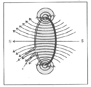
Magnetic field lines provide a powerful way to visualize magnetic fields, just as electric field lines help us understand electric fields. However, magnetic field lines have a crucial difference: they always form closed loops. Unlike electric field lines that begin on positive charges and end on negative charges, magnetic field lines have no beginning or end – they form continuous loops that reveal the fundamental nature of magnetism.
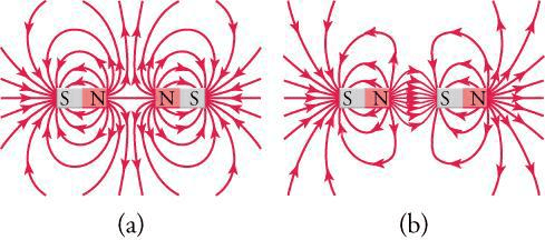
The direction of a magnetic field at any point is defined as the direction a compass needle would point at that location. By convention, magnetic field lines point away from north poles and toward south poles. The density of field lines indicates field strength – where lines are closer together, the magnetic field is stronger.
Real-World Physics: Earth itself acts like a giant bar magnet, with magnetic field lines emerging from the magnetic south pole (near the geographic north pole) and entering at the magnetic north pole (near the geographic south). This is why compass needles point toward magnetic north, which is slightly different from true geographic north.
Magnetic Field Strength and Units
Magnetic field strength is measured in tesla (T), named after the brilliant inventor Nikola Tesla. One tesla is an extremely strong magnetic field – the Earth’s magnetic field is only about 5 × 10⁻⁵ T, while the strongest permanent magnets produce fields of about 1 T. MRI machines use fields of 1-3 T, and the most powerful electromagnets can reach over 40 T.
[EQUATION: Magnetic Field B measured in tesla (T) where 1 T = 1 N/(A·m) = 1 Wb/m²]
The Source of Magnetic Fields
All magnetic fields ultimately arise from moving electric charges. In permanent magnets, atomic-level circulating currents create tiny magnetic dipoles that can align to produce macroscopic magnetic fields. In electromagnets, macroscopic electric currents create controlled magnetic fields that can be turned on and off.
This connection between electricity and magnetism was one of the most important discoveries in physics. What seemed like two separate phenomena – electricity and magnetism – are actually different aspects of the same fundamental force: electromagnetism.
Problem-Solving Strategy: When analyzing magnetic field problems, always start by identifying the source of the magnetic field (permanent magnet, current-carrying wire, etc.) and then determine the geometry of the situation. The mathematical complexity often depends on the symmetry of the configuration.
Key Takeaways:
- Magnetic field lines form closed loops with no beginning or end
- Magnetic field strength is measured in tesla (T)
- All magnetic fields originate from moving electric charges
- Earth’s magnetic field affects compass navigation globally
2: Magnetic Forces on Moving Charges
One of the most fundamental aspects of magnetism is how magnetic fields exert forces on moving electric charges. This force, known as the Lorentz force, forms the basis for countless technologies from electric motors to particle accelerators.
The Lorentz Force Law
When a charged particle moves through a magnetic field, it experiences a force that depends on its charge, velocity, and the magnetic field strength. The mathematical relationship is elegantly simple yet profoundly important:
[EQUATION: Magnetic Force F = q(v × B) where q is charge in coulombs, v is velocity vector in m/s, and B is magnetic field vector in tesla]
For the magnitude of the force when velocity and magnetic field are perpendicular:
[EQUATION: F = qvB sin θ where θ is the angle between velocity and magnetic field vectors]
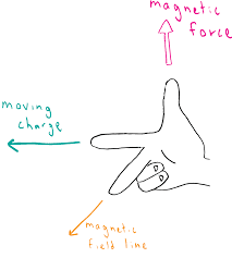
The direction of this force is given by the right-hand rule: point your fingers in the direction of velocity, curl them toward the magnetic field direction, and your thumb points in the direction of force (for positive charges). For negative charges, the force direction is opposite.
Analyzing Particle Motion in Magnetic Fields
When a charged particle moves perpendicular to a uniform magnetic field, something remarkable happens: the magnetic force provides exactly the centripetal force needed for circular motion. The particle follows a circular path with a specific radius and frequency that depend only on the particle’s properties and the magnetic field strength.
Deriving the Circular Motion Equations:
For circular motion: F_centripetal = F_magnetic
mv²/r = qvB
Therefore: r = mv/(qB)
The radius of curvature is independent of the particle’s speed! This surprising result means that faster particles follow larger circles, but the time to complete one orbit remains constant.
[EQUATION: Cyclotron Frequency f = qB/(2πm) where f is frequency in Hz, q is charge, B is magnetic field, and m is particle mass]
Applications of Charged Particle Motion
Mass Spectrometry: By measuring the radius of curvature of ions in a magnetic field, scientists can determine their mass-to-charge ratios. This technique is essential for identifying unknown substances and analyzing molecular structures.
Cyclotron Accelerators: These devices use the constant cyclotron frequency to accelerate particles to high energies. As particles gain energy, their orbits get larger, but their orbital frequency remains constant, allowing synchronized acceleration.
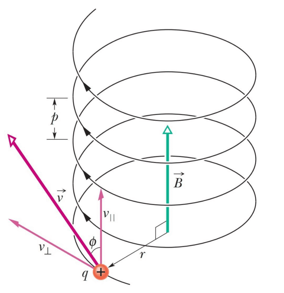
Aurora Formation: The northern and southern lights result from charged particles from the solar wind getting trapped in Earth’s magnetic field. These particles spiral along magnetic field lines and eventually collide with atmospheric gases, creating the beautiful light displays.
Real-World Physics: The Van Allen radiation belts surrounding Earth are regions where charged particles from the solar wind become trapped by Earth’s magnetic field. These particles spiral back and forth between the magnetic poles, creating dangerous radiation zones that spacecraft must navigate carefully.
Worked Example: Electron in a Magnetic Field
An electron with speed 2.0 × 10⁶ m/s enters a uniform magnetic field of 0.50 T perpendicular to its velocity. Calculate the radius of its circular path and the time for one complete orbit.
Solution:
Given:
- q = -1.6 × 10⁻¹⁹ C (electron charge)
- m = 9.1 × 10⁻³¹ kg (electron mass)
- v = 2.0 × 10⁶ m/s
- B = 0.50 T
Step 1: Calculate radius
r = mv/(|q|B) = (9.1 × 10⁻³¹ × 2.0 × 10⁶)/(1.6 × 10⁻¹⁹ × 0.50)
r = 1.82 × 10⁻²⁴/(8.0 × 10⁻²⁰) = 2.3 × 10⁻⁵ m = 23 μm
Step 2: Calculate period
T = 2πm/(|q|B) = (2π × 9.1 × 10⁻³¹)/(1.6 × 10⁻¹⁹ × 0.50)
T = 5.71 × 10⁻³⁰/(8.0 × 10⁻²⁰) = 7.1 × 10⁻¹¹ s
The electron follows a circular path with radius 23 μm and completes one orbit in 71 picoseconds.
Common Error Alert: Students often forget that the magnetic force on a charged particle is always perpendicular to its velocity, which means magnetic fields can change the direction of motion but never change the speed or kinetic energy of a charged particle.
Key Takeaways:
- Magnetic force on moving charges follows F = q(v × B)
- Perpendicular motion results in circular paths with specific radius and frequency
- Particle speed doesn’t affect orbital frequency in uniform magnetic fields
- This principle enables many important technologies and natural phenomena
3: Magnetic Forces on Current-Carrying Wires
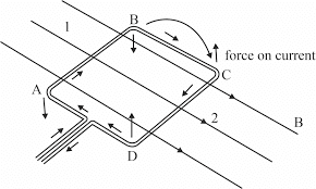
When electric current flows through a wire in the presence of a magnetic field, the moving charges in the current experience magnetic forces that result in a force on the wire itself. This principle forms the foundation for electric motors, speakers, and many other electromagnetic devices.
Force on a Straight Current-Carrying Wire
Consider a straight wire carrying current I through a uniform magnetic field B. The moving charges in the wire experience magnetic forces, and these forces are transmitted to the wire as a whole.
[EQUATION: Force on Wire F = I(L × B) where I is current in amperes, L is length vector of wire in meters, and B is magnetic field in tesla]
For a straight wire perpendicular to a uniform magnetic field:
[EQUATION: F = ILB sin θ where θ is angle between wire direction and magnetic field]
The direction of the force follows the right-hand rule: point your fingers in the direction of conventional current, curl them toward the magnetic field direction, and your thumb indicates the force direction.
The Motor Principle
Electric motors operate on the principle that current-carrying wires experience forces in magnetic fields. A simple motor consists of a current-carrying loop (rotor) in a magnetic field. The forces on opposite sides of the loop create a torque that causes rotation.
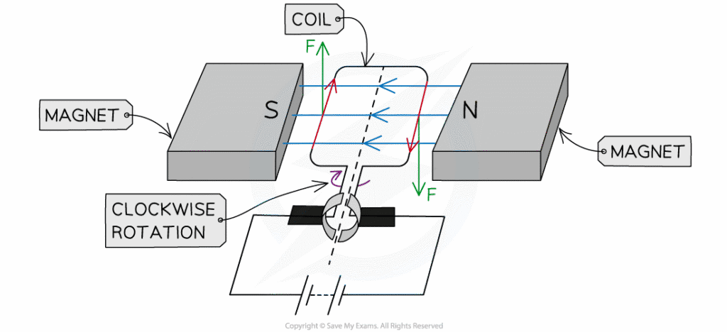
The torque on a current loop in a magnetic field is:
[EQUATION: Torque τ = NIAB sin θ where N is number of turns, I is current, A is loop area, B is magnetic field, and θ is angle between field and loop normal]
Real-World Physics: The speakers in your headphones work on this same principle. Audio signals create varying currents in a coil suspended in a magnetic field. The resulting forces cause the coil (and attached diaphragm) to vibrate, creating sound waves that match the electrical audio signal.
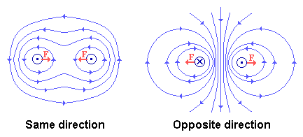
Forces Between Current-Carrying Wires
Two parallel wires carrying current exert magnetic forces on each other. This phenomenon demonstrates that magnetic fields can transmit forces between separate conductors.
For two parallel wires separated by distance d:
[EQUATION: Force per unit length F/L = μ₀I₁I₂/(2πd) where μ₀ = 4π × 10⁻⁷ T·m/A is permeability of free space]
Parallel currents attract; antiparallel currents repel.
This force relationship actually defines the ampere: one ampere is the current that, when flowing through two parallel wires one meter apart, produces a force of 2 × 10⁻⁷ N per meter of wire length.
Worked Example: Motor Torque Calculation
A rectangular current loop with dimensions 10 cm × 15 cm carries a current of 2.0 A and is placed in a uniform magnetic field of 0.80 T. The field is parallel to the 10 cm sides of the loop. Calculate the maximum torque on the loop.
Solution:
Given:
- Length = 0.15 m, Width = 0.10 m
- Area A = 0.15 × 0.10 = 0.015 m²
- Current I = 2.0 A
- Magnetic field B = 0.80 T
- Number of turns N = 1
Maximum torque occurs when θ = 90° (sin θ = 1):
τ_max = NIAB = 1 × 2.0 × 0.015 × 0.80 = 0.024 N·m
The maximum torque on the loop is 0.024 N·m.
Problem-Solving Strategy: When analyzing forces on current-carrying wires, always establish a clear coordinate system and use vector methods when dealing with three-dimensional situations. Remember that magnetic forces are always perpendicular to both the current direction and the magnetic field.
Key Takeaways:
- Current-carrying wires experience forces in magnetic fields according to F = IL × B
- This principle enables electric motors and speakers
- Parallel currents attract; antiparallel currents repel
- Torque on current loops forms the basis for motor operation
4: Sources of Magnetic Fields
Understanding how magnetic fields are created is essential for mastering electromagnetism. While we’ve studied how magnetic fields affect charges and currents, now we explore how moving charges and currents generate magnetic fields.
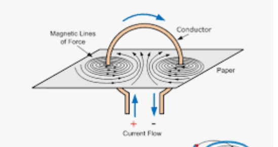
Magnetic Field Around a Straight Current-Carrying Wire
A long, straight wire carrying current produces a magnetic field that forms concentric circles around the wire. The field strength decreases with distance from the wire according to a simple inverse relationship.
[EQUATION: Magnetic Field around Wire B = μ₀I/(2πr) where μ₀ = 4π × 10⁻⁷ T·m/A, I is current, and r is distance from wire]
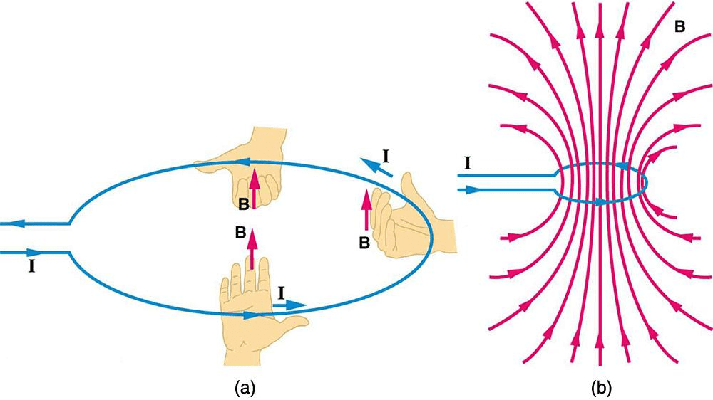
The direction of the magnetic field follows the right-hand rule: point your right thumb in the direction of current flow, and your fingers curl in the direction of the magnetic field lines.
Magnetic Field at the Center of a Current Loop
A circular loop carrying current creates a magnetic field that’s concentrated along the axis of the loop. At the center of the loop, the field is uniform and perpendicular to the loop’s plane.
[EQUATION: Magnetic Field at Loop Center B = μ₀I/(2R) where R is the radius of the loop]
For a coil with N turns:
[EQUATION: B = μ₀NI/(2R)]
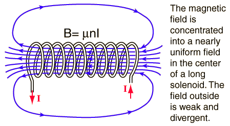
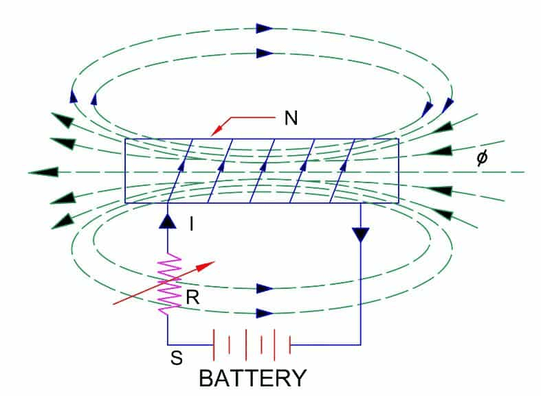
Solenoids: Creating Uniform Magnetic Fields
A solenoid is a long coil of wire that produces a remarkably uniform magnetic field inside the coil. The field inside an ideal solenoid (long compared to its diameter) is:
[EQUATION: Magnetic Field Inside Solenoid B = μ₀nI where n = N/L is turns per unit length]
The magnetic field inside a solenoid is uniform and parallel to the axis, while the field outside is negligible for a long solenoid.
Real-World Physics: MRI machines use superconducting solenoids to create the strong, uniform magnetic fields needed for medical imaging. These solenoids can maintain magnetic fields of 1-3 tesla without any power input once the superconducting state is established.
Ampère’s Circuital Law
Ampère’s law provides an elegant method for calculating magnetic fields in situations with high symmetry. It states that the line integral of the magnetic field around any closed path equals μ₀ times the current enclosed by that path.
[EQUATION: Ampère’s Law ∮ B·dl = μ₀I_enclosed]
This law is particularly useful for calculating fields around:
- Long straight wires (cylindrical symmetry)
- Solenoids (translational symmetry)
- Toroids (rotational symmetry)
Worked Example: Magnetic Field Inside a Solenoid
A solenoid with 1000 turns is 0.50 m long and carries a current of 3.0 A. Calculate the magnetic field inside the solenoid.
Solution:
Given:
- N = 1000 turns
- L = 0.50 m
- I = 3.0 A
- μ₀ = 4π × 10⁻⁷ T·m/A
Step 1: Calculate turns per unit length
n = N/L = 1000/0.50 = 2000 turns/m
Step 2: Apply solenoid field equation
B = μ₀nI = (4π × 10⁻⁷) × 2000 × 3.0
B = 4π × 10⁻⁷ × 6000 = 7.5 × 10⁻³ T = 7.5 mT
The magnetic field inside the solenoid is 7.5 mT.
Common Error Alert: Students often confuse the formulas for magnetic field at the center of a single loop versus inside a solenoid. Remember: single loop uses B = μ₀I/(2R), while solenoid uses B = μ₀nI.
Physics Check: A current-carrying wire produces what kind of magnetic field pattern?
Answer: Concentric circles around the wire, with field strength decreasing as 1/r.
Key Takeaways:
- Moving charges and electric currents create magnetic fields
- Field patterns depend on current geometry (straight wire, loop, solenoid)
- Ampère’s law provides an elegant method for high-symmetry situations
- Solenoids create uniform magnetic fields essential for many applications
5: Electromagnetic Induction – The Heart of Modern Technology
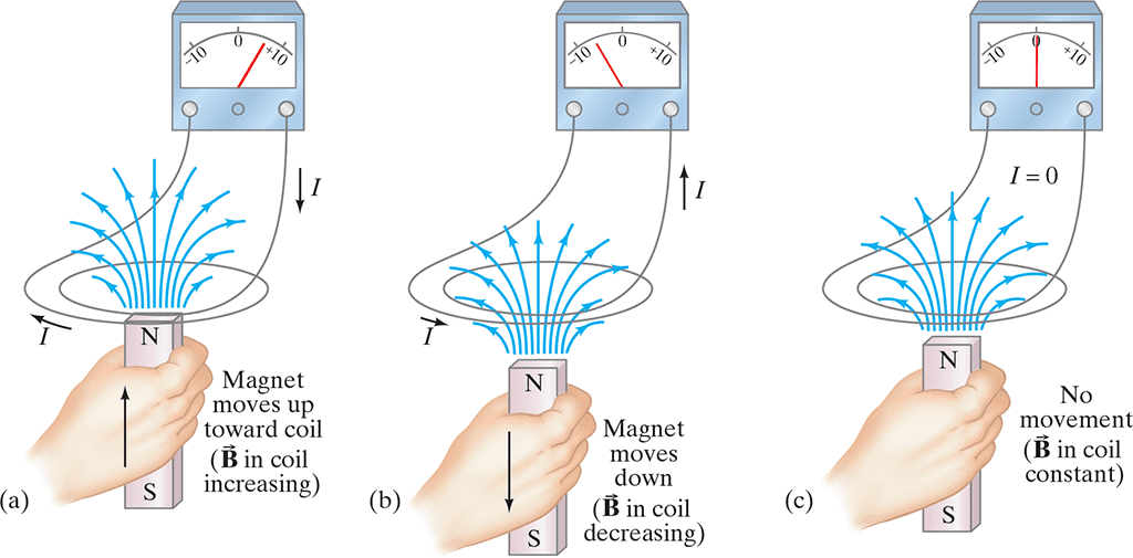
Electromagnetic induction represents one of the most profound discoveries in physics. Michael Faraday’s 1831 discovery that changing magnetic fields can induce electric currents revolutionized our understanding of electromagnetism and laid the foundation for generators, transformers, and countless modern technologies.
Faraday’s Law of Electromagnetic Induction
Faraday discovered that a changing magnetic flux through a loop of wire induces an electromotive force (EMF) in the loop. This relationship is quantified by Faraday’s law:
[EQUATION: Faraday’s Law ε = -N(dΦ_B/dt) where ε is induced EMF, N is number of turns, and Φ_B is magnetic flux]
Magnetic flux is defined as:
[EQUATION: Magnetic Flux Φ_B = B·A = BA cos θ where B is magnetic field, A is area vector, and θ is angle between them]
The negative sign in Faraday’s law reflects Lenz’s law, which we’ll explore in detail shortly.
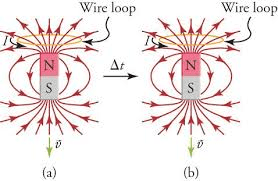
Understanding Magnetic Flux
Think of magnetic flux as the “amount” of magnetic field passing through a surface. Just as water flux through a window depends on both the water flow rate and the window’s area and orientation, magnetic flux depends on the magnetic field strength, the loop area, and their relative orientation.
Ways to Change Magnetic Flux:
- Change the magnetic field strength (B changes)
- Change the loop area (A changes)
- Change the orientation (θ changes)
- Move the loop to a different field region
Each of these changes can induce an EMF according to Faraday’s law.
Lenz’s Law: Nature’s Opposition to Change
Heinrich Lenz formulated a rule for determining the direction of induced currents: the induced current flows in such a direction that its magnetic field opposes the change that produced it. This is a manifestation of energy conservation – if induced currents aided the change that created them, we could extract unlimited energy from electromagnetic systems.
[EQUATION: Lenz’s Law: Induced effects oppose the changes that cause them]
Applying Lenz’s Law:
- Identify what’s changing (increasing/decreasing flux)
- Determine what would oppose this change
- Find the current direction that creates the opposing effect
Real-World Physics: Lenz’s law explains why dropping a magnet through a copper tube takes much longer than dropping it through air. The changing magnetic flux as the magnet falls induces currents in the copper that create magnetic fields opposing the magnet’s motion, effectively creating a “magnetic drag” force.
Motional EMF: Moving Conductors in Magnetic Fields
When a conductor moves through a magnetic field, the magnetic force on the mobile charges in the conductor creates a separation of charge, resulting in an induced EMF. This motional EMF forms the basis for many practical applications.
For a straight conductor of length L moving with velocity v perpendicular to magnetic field B:
[EQUATION: Motional EMF ε = BLv]
Worked Example: Generator Analysis
A rectangular coil with 50 turns, each with area 0.20 m², rotates at 60 Hz in a uniform magnetic field of 0.15 T. Calculate the maximum induced EMF.
Solution:
Given:
- N = 50 turns
- A = 0.20 m²
- f = 60 Hz, so ω = 2πf = 2π(60) = 377 rad/s
- B = 0.15 T
For a rotating coil: Φ(t) = NBA cos(ωt)
The induced EMF is:
ε = -N(dΦ/dt) = -N(-NBA ω sin(ωt)) = NBAω sin(ωt)
Maximum EMF occurs when sin(ωt) = 1:
ε_max = NBAω = 50 × 0.15 × 0.20 × 377 = 566 V
The maximum induced EMF is 566 V.
Problem-Solving Strategy: When solving induction problems, always start by identifying what quantity is changing and how it changes with time. Then apply Faraday’s law systematically, being careful about signs and directions.
Key Takeaways:
- Faraday’s law quantifies electromagnetic induction: ε = -N(dΦ_B/dt)
- Magnetic flux can change through field, area, or orientation changes
- Lenz’s law determines the direction of induced effects
- Motional EMF occurs when conductors move through magnetic fields
6: AC Generators and Transformers
The practical applications of electromagnetic induction include some of the most important devices in modern society. Generators convert mechanical energy to electrical energy, while transformers allow efficient transmission and distribution of electrical power.
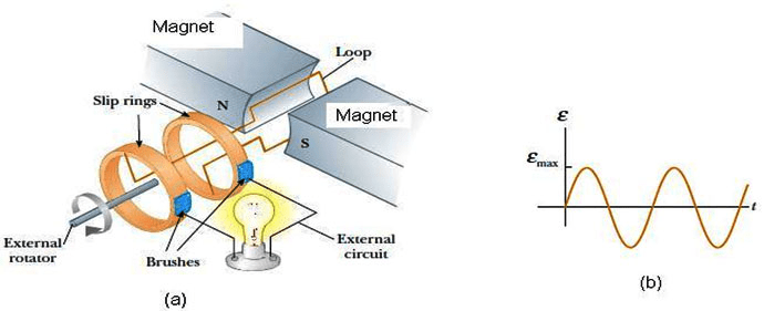
AC Generator Operation
An AC generator (alternator) consists of a coil rotating in a magnetic field. As the coil rotates, the magnetic flux through it changes sinusoidally, producing a sinusoidal EMF.
For a coil with N turns, area A, rotating at angular frequency ω in magnetic field B:
[EQUATION: Generated EMF ε(t) = NBAω sin(ωt) = ε_max sin(ωt)]
The maximum EMF is:
[EQUATION: ε_max = NBAω]
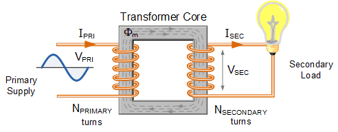
Transformer Principles
Transformers use electromagnetic induction to change AC voltage levels. They consist of two coils (primary and secondary) wound around a common iron core. The changing current in the primary coil creates a changing magnetic flux that induces EMF in the secondary coil.
[EQUATION: Transformer Voltage Relation V_s/V_p = N_s/N_p where subscripts s and p refer to secondary and primary]
For an ideal transformer (100% efficiency):
[EQUATION: Power Conservation P_p = P_s, so I_s/I_p = N_p/N_s]
Step-up transformer: N_s > N_p (increases voltage, decreases current)
Step-down transformer: N_s < N_p (decreases voltage, increases current)
Real-World Physics: The electrical grid uses transformers extensively. Power plants generate electricity at relatively low voltages (thousands of volts), which is stepped up to very high voltages (hundreds of thousands of volts) for long-distance transmission to minimize power losses. Near your home, transformers step the voltage back down to the 120V/240V used in household circuits.
Energy Considerations in Electromagnetic Induction
Electromagnetic induction always involves energy conversion. In generators, mechanical energy converts to electrical energy. In transformers, electrical energy at one voltage level converts to electrical energy at another voltage level.
Lenz’s law ensures energy conservation: The induced effects always oppose the changes that cause them, which means work must be done to maintain the changing conditions that produce induction.
Worked Example: Transformer Design
A transformer is needed to operate a 24V, 60W device from a 120V AC supply. Calculate the required turns ratio and the primary current.
Solution:
Given:
- V_p = 120 V (primary voltage)
- V_s = 24 V (secondary voltage)
- P_s = 60 W (secondary power)
Step 1: Calculate turns ratio
N_s/N_p = V_s/V_p = 24/120 = 1/5 = 0.20
This is a step-down transformer with a 5:1 turns ratio.
Step 2: Calculate secondary current
I_s = P_s/V_s = 60/24 = 2.5 A
Step 3: Calculate primary current (assuming ideal transformer)
I_p = I_s × (N_s/N_p) = 2.5 × 0.20 = 0.50 A
The transformer needs a 5:1 turns ratio, and the primary current will be 0.50 A.
Common Error Alert: Students often confuse the relationship between turns ratio and voltage/current ratios in transformers. Remember: voltage ratios equal turns ratios, but current ratios are inverted from turns ratios.
Key Takeaways:
- AC generators convert mechanical energy to electrical energy through rotating coils
- Generated EMF varies sinusoidally with time
- Transformers change AC voltage levels using electromagnetic induction
- Energy conservation governs all electromagnetic induction processes
7: Self-Inductance and Inductors
When current flows through a coil, it creates a magnetic field that passes through the coil itself. Any change in this current changes the magnetic flux through the coil, which induces an EMF that opposes the current change. This phenomenon, called self-inductance, is crucial for understanding many electrical circuits.
Understanding Self-Inductance
Self-inductance (L) is a measure of how much EMF is induced in a coil when its current changes. It depends only on the physical properties of the coil: its geometry, number of turns, and the permeability of its core material.
[EQUATION: Self-Induced EMF ε = -L(dI/dt) where L is inductance in henries (H)]
The inductance of a solenoid is:
[EQUATION: Solenoid Inductance L = μ₀n²Al where n is turns per unit length, A is cross-sectional area, and l is length]
Energy Stored in Inductors
Like capacitors store energy in electric fields, inductors store energy in magnetic fields. The energy stored in an inductor carrying current I is:
[EQUATION: Energy in Inductor U = ½LI²]
This energy is stored in the magnetic field created by the current. When the current changes, this energy can be released back to the circuit.
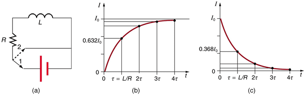
RL Circuits: Inductors with Resistors
When an inductor is connected to a DC source through a resistor, the current doesn’t jump immediately to its steady-state value. Instead, it grows exponentially with a characteristic time constant.
[EQUATION: Time Constant τ = L/R]
Current Growth: I(t) = (ε/R)(1 – e^(-t/τ))
Current Decay: I(t) = I₀e^(-t/τ)
Real-World Physics: Inductors in car ignition systems store energy when current flows through them. When the current is suddenly interrupted, the collapsing magnetic field induces a very high voltage that creates the spark needed to ignite the fuel-air mixture in the engine cylinders.
Worked Example: RL Circuit Analysis
An inductor with L = 50 mH is connected in series with a 100 Ω resistor and a 12 V battery. Calculate the time constant and the current 0.25 ms after the switch is closed.
Solution:
Given:
- L = 50 × 10⁻³ H
- R = 100 Ω
- ε = 12 V
- t = 0.25 × 10⁻³ s
Step 1: Calculate time constant
τ = L/R = (50 × 10⁻³)/100 = 5.0 × 10⁻⁴ s = 0.50 ms
Step 2: Calculate steady-state current
I_steady = ε/R = 12/100 = 0.12 A
Step 3: Calculate current at t = 0.25 ms
I(t) = I_steady(1 – e^(-t/τ))
I(0.25 ms) = 0.12(1 – e^(-0.25/0.50)) = 0.12(1 – e^(-0.5))
I(0.25 ms) = 0.12(1 – 0.606) = 0.12(0.394) = 0.047 A
The time constant is 0.50 ms, and the current after 0.25 ms is 0.047 A.
Key Takeaways:
- Self-inductance opposes changes in current through coils
- Inductors store energy in magnetic fields
- RL circuits exhibit exponential current changes with time constant τ = L/R
- Self-inductance is crucial for many electrical devices and circuits
8: Laboratory Investigations and Experimental Design
Laboratory work in electromagnetism provides hands-on experience with the concepts you’ve studied theoretically. The College Board emphasizes experimental design, data analysis, and connecting laboratory observations to theoretical principles.
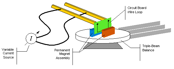
Investigation 1: Magnetic Force on Current-Carrying Wire
This investigation explores how magnetic force depends on current, magnetic field strength, and wire orientation.
Experimental Setup:
A current-carrying wire is placed in a known magnetic field, and the magnetic force is measured using a sensitive balance or force sensor.
Variables to Investigate:
- Independent variables: Current magnitude, wire length in field, angle between wire and field
- Dependent variable: Magnetic force
- Control variables: Temperature, wire material, magnetic field uniformity
Expected Relationships:
- Force should be proportional to current: F ∝ I
- Force should be proportional to wire length: F ∝ L
- Force should vary as sin θ with angle
Data Analysis:
Plot force vs. current to verify linear relationship and determine the slope, which equals BL for perpendicular orientation. Compare experimental slope to calculated value using known B and measured L.
Sources of Error:
- Magnetic field non-uniformity
- Temperature effects on wire resistance
- Mechanical vibrations affecting force measurements
- Earth’s magnetic field contributions
Investigation 2: Electromagnetic Induction
This investigation demonstrates Faraday’s law by measuring induced EMF as magnetic flux changes through a coil.
Experimental Design:
Move a strong magnet toward and away from a coil connected to a sensitive voltmeter or oscilloscope.
Quantitative Measurements:
- Vary magnet speed and measure peak induced EMF
- Use different numbers of coil turns
- Change magnet strength and orientation
- Measure EMF as function of distance from coil
Testing Faraday’s Law:
The relationship ε = -N(dΦ/dt) can be tested by:
- Verifying EMF proportional to number of turns (N)
- Confirming EMF proportional to rate of flux change (dΦ/dt)
- Checking sign relationship (Lenz’s law)
Advanced Analysis:
Use motion sensors to measure magnet velocity simultaneously with EMF measurements. Calculate expected flux change rate and compare to measured EMF.
Investigation 3: AC Generator Simulation
Build a simple AC generator and investigate how design parameters affect the generated EMF.
Construction:
- Rotating coil in magnetic field
- Slip rings for electrical connection
- Variable speed motor for controlled rotation
- Magnetic field from permanent magnets or electromagnets
Parameters to Vary:
- Rotation frequency (ω)
- Number of coil turns (N)
- Coil area (A)
- Magnetic field strength (B)
Measurements:
- EMF amplitude vs. rotation frequency
- EMF frequency vs. rotation frequency
- Effect of coil parameters on EMF amplitude
Data Analysis:
Verify the relationship ε_max = NBAω by plotting maximum EMF against each parameter while holding others constant. The slopes of these plots should match theoretical predictions.
Experimental Design Skills
Planning Effective Investigations:
- Clear objectives: What specific relationship are you testing?
- Variable identification: Independent, dependent, and control variables
- Range and precision: Appropriate measurement ranges and uncertainties
- Multiple trials: Statistical analysis and uncertainty assessment
- Systematic approach: Logical sequence of measurements
Data Collection Best Practices:
- Record environmental conditions (temperature, humidity)
- Note any unusual observations or equipment behavior
- Take multiple measurements for statistical analysis
- Document equipment specifications and calibration
Error Analysis:
- Random errors: Use multiple trials and statistical analysis
- Systematic errors: Consider equipment limitations and environmental factors
- Uncertainty propagation: Calculate how measurement uncertainties affect final results
Physics Check: Design an experiment to verify that the magnetic force on a current-carrying wire is perpendicular to both the current direction and the magnetic field.
Key elements:
- Method for varying current direction and magnetic field orientation
- Force measurement technique sensitive to direction
- Control of other variables that might affect force magnitude
- Data analysis approach to confirm perpendicular relationship
Key Takeaways:
- Laboratory work reinforces theoretical understanding of electromagnetic principles
- Experimental design requires careful consideration of variables and errors
- Quantitative measurements should be compared to theoretical predictions
- Error analysis and uncertainty assessment are essential skills
9: Practice Problems – Mastering Electromagnetic Concepts
Let’s apply your understanding with comprehensive practice problems that reflect the style and complexity of AP Physics 2 exam questions.
Multiple Choice Questions
Question 1: A charged particle moves in a circular path of radius R in a uniform magnetic field. If the particle’s speed doubles while the magnetic field remains constant, the new radius becomes:
A) R/4
B) R/2
C) R
D) 2R
Solution: Using r = mv/(qB), if v doubles and B is constant, then r doubles.
Answer: D
Question 2: A rectangular loop of wire moves at constant velocity into a region of uniform magnetic field. While the loop is entering the field region, the induced current:
A) Is zero because velocity is constant
B) Flows clockwise when viewed from above
C) Flows counterclockwise when viewed from above
D) Direction depends on the loop’s orientation
Solution: Apply Lenz’s law: as flux through the loop increases (more field lines entering), the induced current must create a magnetic field opposing this increase. By the right-hand rule, current flows counterclockwise to create an upward magnetic field opposing the downward applied field.
Answer: C
Question 3: An ideal transformer has 100 turns in its primary coil and 25 turns in its secondary coil. If the primary current is 2.0 A, the secondary current is:
A) 0.5 A
B) 2.0 A
C) 4.0 A
D) 8.0 A
Solution: For ideal transformers: I_s/I_p = N_p/N_s = 100/25 = 4
Therefore: I_s = 4 × 2.0 = 8.0 A
Answer: D
Free Response Problems
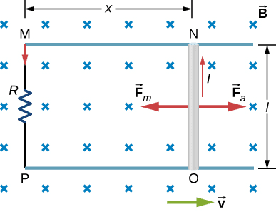
Problem 4: A conducting rod of length 0.50 m slides along two parallel conducting rails separated by the same distance. The rails are connected by a resistor and placed in a uniform magnetic field of 0.20 T perpendicular to the plane of the rails. The rod moves at constant velocity of 3.0 m/s.
(a) Calculate the motional EMF induced in the rod.
(b) If the total resistance of the circuit is 0.60 Ω, find the induced current.
(c) Determine the magnetic force on the rod and explain why external force is needed to maintain constant velocity.
(d) Calculate the power dissipated in the resistor and show that it equals the mechanical power input.
Solution:
(a) Motional EMF: ε = BLv = 0.20 × 0.50 × 3.0 = 0.30 V
(b) Induced current: I = ε/R = 0.30/0.60 = 0.50 A
(c) Magnetic force on rod: F = BIL = 0.20 × 0.50 × 0.50 = 0.050 N
By Lenz’s law, this force opposes the motion. An external force of 0.050 N is needed to maintain constant velocity.
(d) Power dissipated: P_resistor = I²R = (0.50)² × 0.60 = 0.15 W
Mechanical power input: P_mechanical = F_external × v = 0.050 × 3.0 = 0.15 W
The powers are equal, confirming energy conservation.
Problem 5: A solenoid with 500 turns, length 0.40 m, and cross-sectional area 0.020 m² carries a current that increases linearly from 0 to 2.0 A in 50 ms.
(a) Calculate the inductance of the solenoid.
(b) Find the self-induced EMF during the current increase.
(c) Determine the energy stored in the magnetic field when the current reaches 2.0 A.
Solution:
(a) Solenoid inductance:
n = N/l = 500/0.40 = 1250 turns/m
L = μ₀n²Al = (4π × 10⁻⁷) × (1250)² × 0.020 × 0.40
L = (4π × 10⁻⁷) × 1.56 × 10⁶ × 0.008 = 1.56 × 10⁻² H = 15.6 mH
(b) Self-induced EMF:
dI/dt = ΔI/Δt = (2.0 – 0)/(50 × 10⁻³) = 40 A/s
ε = -L(dI/dt) = -0.0156 × 40 = -0.624 V
The magnitude of self-induced EMF is 0.624 V.
(c) Energy stored:
U = ½LI² = ½ × 0.0156 × (2.0)² = 0.031 J
Data Analysis Problem
Problem 6: Students investigate the relationship between magnetic field strength and the radius of curvature for electrons in a cathode ray tube. Their data is shown below:
| Magnetic Field (mT) | Radius (cm) |
|---|---|
| 0.50 | 11.4 |
| 1.00 | 5.7 |
| 1.50 | 3.8 |
| 2.00 | 2.9 |
| 2.50 | 2.3 |
(a) What relationship should exist between B and r according to theory?
(b) Plot an appropriate graph to test this relationship.
(c) From the graph, determine the electron’s speed.
(d) Calculate the expected radius for B = 3.0 mT.
Solution:
(a) From r = mv/(qB), we expect r ∝ 1/B, or r = (mv/q) × (1/B)
(b) Plot 1/r vs. B should give a straight line with slope q/(mv)
(c) From the graph slope and known electron properties:
Slope = q/(mv) = (1.6 × 10⁻¹⁹)/(9.1 × 10⁻³¹ × v)
Using experimental slope ≈ 1.75 × 10⁴ (1/T·m):
v = (1.6 × 10⁻¹⁹)/(9.1 × 10⁻³¹ × 1.75 × 10⁴) = 1.0 × 10⁷ m/s
(d) For B = 3.0 mT:
r = mv/(qB) = (9.1 × 10⁻³¹ × 1.0 × 10⁷)/(1.6 × 10⁻¹⁹ × 3.0 × 10⁻³) = 1.9 cm
Experimental Design Question
Problem 7: Design an experiment to determine the relationship between the number of turns in a solenoid and the magnetic field at its center.
Required elements:
- Experimental setup and equipment
- Variables and controls
- Measurement procedures
- Data analysis methods
- Error sources and minimization strategies
Sample Response Framework:
Setup: Variable solenoids (different turn counts) with same geometry, DC power supply, Hall probe or compass for field measurement, current meter.
Variables:
- Independent: Number of turns (N)
- Dependent: Magnetic field at center (B)
- Controls: Current, solenoid length, core material, temperature
Procedure:
- Construct solenoids with different turn counts using same wire gauge and length
- Pass identical current through each solenoid
- Measure magnetic field at geometric center using Hall probe
- Repeat measurements with multiple current values
- Plot B vs. N for each current value
Expected Results: Linear relationship B = (μ₀I/2R) × N
Error Minimization:
- Precise positioning of field probe at solenoid center
- Multiple measurements at each data point
- Careful current regulation and measurement
- Account for Earth’s magnetic field background
Physics Check: Quick verification questions:
- What creates magnetic fields around current-carrying wires?
- How does Lenz’s law relate to energy conservation?
- Why do transformers only work with AC, not DC?
- What happens to inductance if you double the number of turns in a coil?
Key Takeaways:
- Practice problems integrate multiple electromagnetic concepts
- Experimental design questions test deep understanding of principles
- Data analysis skills are essential for quantitative physics
- Problem-solving strategies should be systematic and thorough
10: Exam Strategies and Common Pitfalls
Success on AP Physics 2 electromagnetic questions requires strategic thinking, careful analysis, and awareness of common mistakes that trap even well-prepared students.
Understanding AP Physics 2 Electromagnetic Question Types
Conceptual Understanding Questions:
These test your grasp of fundamental principles without extensive calculations. Focus on:
- Direction of magnetic forces and fields (right-hand rules)
- Lenz’s law applications
- Energy conservation in electromagnetic systems
- Cause-and-effect relationships in induction
Quantitative Problem-Solving:
These require systematic application of equations and mathematical reasoning:
- Force calculations on charges and currents
- Magnetic field calculations from various current configurations
- EMF calculations using Faraday’s law
- Circuit analysis with inductors
Experimental Design and Analysis:
These assess your ability to plan investigations and interpret data:
- Designing experiments to test electromagnetic principles
- Analyzing experimental data and identifying relationships
- Evaluating sources of error and uncertainty
- Connecting experimental results to theoretical concepts
Strategic Approaches to Different Problem Types
Strategy 1: Magnetic Force Problems
Common Question Pattern: “A charged particle or current-carrying wire experiences a force in a magnetic field. Find the force magnitude and direction.”
Systematic Approach:
- Identify the situation: Moving charge or current in external field
- Choose appropriate equation: F = q(v × B) or F = I(L × B)
- Apply right-hand rule: Determine force direction
- Calculate magnitude: Use F = qvB sin θ or F = ILB sin θ
- Check reasonableness: Force should be perpendicular to both v (or I) and B
Common Error Alert: Students often forget that magnetic force is always perpendicular to velocity, which means it changes direction but never changes speed or kinetic energy of a charged particle.
Strategy 2: Electromagnetic Induction Problems
Common Question Pattern: “A conductor moves through a magnetic field, or a magnetic field changes near a conductor. Find the induced EMF and current.”
Step-by-Step Method:
- Identify what’s changing: Flux due to motion, field change, or area change
- Calculate flux change: ΔΦ = Δ(BA cos θ)
- Apply Faraday’s law: ε = -N(ΔΦ/Δt)
- Use Lenz’s law: Determine current direction that opposes the change
- Find current: I = ε/R if resistance is given
Strategy 3: Energy and Power in Electromagnetic Systems
Common Question Pattern: “Analyze energy transformations in generators, motors, or induction systems.”
Key Principles:
- Energy is always conserved
- Mechanical power input equals electrical power output (ideal systems)
- Lenz’s law ensures energy conservation by opposing changes
- Power dissipation: P = I²R = ε²/R
Common Misconceptions and Corrections
Misconception 1: “Magnetic forces can do work on charged particles.”
Reality: Magnetic forces are always perpendicular to velocity, so they can’t change kinetic energy. They can change direction of motion but not speed.
Misconception 2: “Lenz’s law means induced currents always oppose applied currents.”
Reality: Lenz’s law means induced effects oppose the changes that cause them, not necessarily the applied fields or currents themselves.
Misconception 3: “Transformers work with DC because they use magnetic fields.”
Reality: Transformers require changing magnetic fields to induce EMF. DC produces constant magnetic fields, so no induction occurs.
Misconception 4: “Stronger magnets always produce larger forces.”
Reality: Magnetic force depends on the relative orientation of velocity (or current) and magnetic field. Maximum force occurs when they’re perpendicular.
Real-World Physics: Remember that electromagnetic principles govern countless technologies around you. When you understand how a problem relates to familiar devices (motors, generators, transformers, MRI machines), you often gain insight into the correct approach.
Conclusion: Mastering Electromagnetism and Its Applications
Congratulations on completing this comprehensive journey through AP Physics 2 Unit 12: Magnetism and Electromagnetism. You’ve explored one of the most elegant and practically important areas of physics – the intricate relationship between electric and magnetic phenomena that powers our modern technological world.
Conceptual Mastery Review
You now understand the fundamental principles that govern electromagnetic interactions:
Magnetic Fields and Forces: You’ve learned that magnetic fields arise from moving charges and exert forces on other moving charges according to precise mathematical relationships. These forces, always perpendicular to both velocity and magnetic field, govern everything from the path of cosmic rays to the operation of particle accelerators.
Electromagnetic Induction: Faraday’s discovery that changing magnetic fields induce electric fields (and vice versa) revealed the deep connection between electricity and magnetism. This principle, quantified by Faraday’s law and directed by Lenz’s law, enables generators, transformers, and countless other technologies that define modern life.
Energy and Conservation: Throughout electromagnetism, energy conservation provides both a guiding principle and a powerful problem-solving tool. Lenz’s law itself is a manifestation of energy conservation – if induced effects aided rather than opposed the changes that created them, we could create energy from nothing.
Symmetry and Elegance: The mathematical relationships in electromagnetism reveal deep symmetries in nature. Moving charges create magnetic fields; changing magnetic fields create electric fields. This reciprocal relationship culminates in electromagnetic waves – a topic you’ll explore further in advanced physics courses.
Real-World Applications and Career Connections
The principles you’ve mastered connect directly to numerous career fields and technological applications:
Electrical Engineering: Power generation, transmission, and motor design all rely heavily on electromagnetic principles. Understanding induction is essential for designing efficient transformers and generators.
Medical Technology: MRI machines use powerful magnetic fields and electromagnetic induction to create detailed images of the human body. Pacemakers use electromagnetic principles to regulate heart rhythms.
Transportation: Electric and hybrid vehicles depend on electromagnetic motors and generators. Magnetic levitation trains use magnetic forces to achieve friction-free, high-speed transportation.
Communications: Radio, television, cell phones, and wireless internet all use electromagnetic waves. Understanding basic electromagnetic principles provides the foundation for more advanced studies in telecommunications.
Research and Development: Particle accelerators, fusion reactors, and quantum devices all exploit electromagnetic phenomena. Many cutting-edge technologies require deep understanding of electromagnetic principles.
Looking Ahead: Advanced Electromagnetic Concepts
The principles you’ve learned provide the foundation for more advanced topics you might encounter in college physics or engineering courses:
Maxwell’s Equations: The four fundamental equations that completely describe electromagnetic phenomena, including the prediction of electromagnetic waves.
Electromagnetic Waves: Light, radio waves, X-rays, and all other electromagnetic radiation arise from accelerating charges and propagate according to electromagnetic principles.
Quantum Electrodynamics: The quantum mechanical description of electromagnetic interactions, which explains phenomena that classical physics cannot address.
Plasma Physics: The study of ionized gases where electromagnetic forces dominate, important for fusion energy and space physics.
Study Strategies for Long-Term Retention
Active Connection-Making: Regularly connect electromagnetic principles to phenomena you observe in daily life. When you see electric motors, transformers, or wireless charging, think about the physics principles involved.
Cross-Unit Integration: Electromagnetic concepts connect to many other physics areas. Energy conservation links to thermodynamics; wave properties connect to optics; circular motion principles apply to charged particles in magnetic fields.
Mathematical Fluency: Continue developing your vector analysis and calculus skills. Advanced electromagnetic applications require sophisticated mathematical tools.
Experimental Thinking: Always consider how electromagnetic principles could be tested experimentally. This mindset will serve you well in laboratory courses and research experiences.
The Beauty and Unity of Physics
Electromagnetism exemplifies the beauty and unity that characterize the deepest physics principles. The same mathematical relationships that describe a compass needle aligning with Earth’s magnetic field also govern the operation of the Large Hadron Collider. The induction principles discovered by Faraday in simple laboratory demonstrations now enable the global electrical grid that powers modern civilization.
As you continue your physics education, you’ll discover that electromagnetic principles appear throughout many areas of science. From the quantum mechanics of atoms to the general relativity of black holes, electromagnetic interactions play crucial roles in our understanding of the universe.
Final Thoughts and Encouragement
Mastering electromagnetism represents a significant achievement in your physics education. You’ve developed not just knowledge of specific concepts, but also problem-solving skills, experimental reasoning abilities, and mathematical fluency that will serve you throughout your scientific career.
Whether you pursue engineering, medicine, research, or any field that values quantitative reasoning, the analytical skills you’ve developed while studying electromagnetism will be invaluable. The ability to visualize three-dimensional relationships, apply conservation principles, and connect theoretical concepts to practical applications represents exactly the kind of thinking that drives innovation and discovery.
Remember that every expert was once a beginner, and every breakthrough in electromagnetic technology built upon the fundamental principles you now understand. From Faraday’s early experiments with coils and magnets to the development of wireless power transmission and quantum computers, progress in electromagnetism has always required the same combination of theoretical understanding and practical problem-solving that you’ve been developing.
As you prepare for your AP Physics 2 exam and plan your future studies, take pride in the sophisticated understanding you’ve developed. You now possess the conceptual tools to understand a vast range of phenomena, from the northern lights dancing in Earth’s magnetic field to the electromagnetic waves carrying this message to your screen.
The future of technology – from fusion energy to quantum computers to space exploration – will continue to rely on electromagnetic principles. By mastering these concepts now, you’re preparing yourself to contribute to the next generation of scientific and technological advances.
Keep questioning, keep learning, and remember that the elegant mathematical relationships governing electromagnetism reflect some of the deepest and most beautiful patterns in the natural world. Your understanding of these principles connects you to centuries of scientific discovery and positions you to participate in the exciting developments yet to come.
Good luck with your continued physics journey, and may your understanding of electromagnetism illuminate both your exam success and your future scientific endeavors!
Recommended –
2 thoughts on “AP Physics 2 Unit 12: Magnetism and Electromagnetism – Complete Study Guide (2025)”