Magnetism and Matter Class 12 Notes: NCERT Solutions, Important Questions for CBSE Board Exams 2026

Magnetism in Your Daily Life

Every morning when you use your smartphone’s compass to find directions, stick a note on your refrigerator, or tap your credit card for payment, you’re experiencing the incredible world of magnetism and matter. But have you ever wondered why some materials are attracted to magnets while others aren’t? Why does iron get magnetized but copper doesn’t?

Welcome to Chapter 5 of CBSE Class 12 Physics – a fascinating journey into how different materials respond to magnetic fields. This isn’t just theory you’ll forget after exams. From MRI machines that save lives to the magnetic storage in your laptop, understanding magnetism and matter opens doors to comprehending the technology that surrounds us.

Think about it: Earth itself is a giant magnet that has been guiding travelers for centuries. The Aurora Borealis dancing across polar skies? That’s charged particles interacting with Earth’s magnetic field. Even your body contains iron that responds to strong magnetic fields – that’s how MRI scanners can peek inside you without surgery.

This chapter will transform your understanding of materials from the atomic level up, showing you why a paperclip jumps toward a magnet but a piece of aluminum barely moves. You’ll discover the hidden magnetic properties in everything around you and learn to predict how different substances behave in magnetic fields.

Learning Objectives: Your Roadmap to Mastery

By the end of this comprehensive guide, you’ll confidently:

Classify any material as diamagnetic, paramagnetic, or ferromagnetic based on its atomic structure
Calculate magnetic susceptibility and permeability for different materials
Explain why ferromagnetic materials can become permanent magnets
Analyze hysteresis loops and determine energy losses in magnetic materials
Solve complex numerical problems involving Earth’s magnetic field elements
Design experiments to measure magnetic properties of materials
Connect magnetic concepts to real-world applications in technology and medicine
Score maximum marks in CBSE board exam questions on magnetism and matter

Real-World Physics: Did you know that birds navigate using Earth’s magnetic field? They have magnetic crystals in their beaks that act like biological compasses, helping them migrate thousands of miles with pinpoint accuracy.

Section 1: The Atomic Foundation of Magnetism

Understanding Magnetic Behavior from Atoms Up

Every atom is essentially a tiny magnet, but most materials don’t appear magnetic. This seeming contradiction holds the key to understanding magnetism and matter. Let’s start with what makes an atom magnetic.

When electrons orbit the nucleus, they create tiny circular currents. According to Ampère’s law, any current loop generates a magnetic field, making each orbiting electron a microscopic magnet. Additionally, electrons possess an intrinsic property called spin, which contributes another magnetic moment.

[EQUATION: Orbital Magnetic Moment: μₗ = -μB√[l(l+1)] where μB = eh/4πmₑ = 9.27 × 10⁻²⁴ A⋅m² (Bohr magneton)]

[EQUATION: Spin Magnetic Moment: μₛ = -gₛμB√[s(s+1)] where gₛ ≈ 2 and s = ½ for electrons]

The crucial insight is this: in atoms with completely filled electron shells, all magnetic moments cancel out perfectly. It’s like having equal numbers of people walking clockwise and counterclockwise around a track – the net effect is zero motion.

Physics Check: Can you explain why helium (atomic number 2) with its two electrons in the 1s orbital shows no net magnetic moment?

The Three Magnetic Personalities

Based on how atoms combine their magnetic moments, all materials fall into three distinct categories:

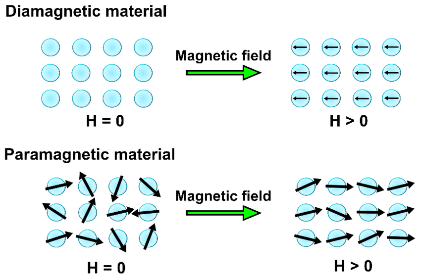
Diamagnetic Materials have no unpaired electrons. When you apply a magnetic field, it induces tiny currents that oppose the field (Lenz’s law in action). These materials are weakly repelled by magnets.

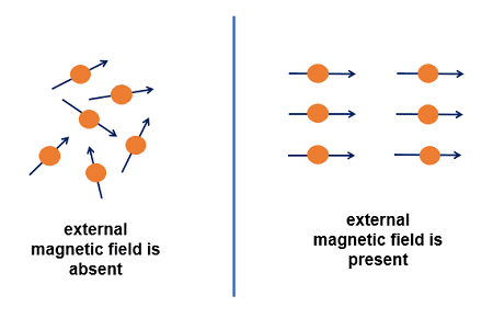
Paramagnetic Materials contain unpaired electrons, giving them permanent atomic magnetic moments. However, thermal motion randomizes these orientations, so they show only weak attraction to magnets.

Ferromagnetic Materials not only have unpaired electrons but also exhibit a quantum mechanical exchange interaction that aligns neighboring atomic magnets even without external fields.

[INSERT DIAGRAM: Three atomic representations showing paired electrons (diamagnetic), unpaired electrons randomly oriented (paramagnetic), and aligned unpaired electrons (ferromagnetic)

Section 2: Mathematical Framework of Magnetic Materials

Magnetic Susceptibility – The Material’s Magnetic Fingerprint

Magnetic susceptibility (χ) tells you exactly how a material responds to magnetic fields. It’s defined as the ratio of magnetization to the magnetic field intensity:

[EQUATION: χ = M/H where M is magnetization (magnetic moment per unit volume) and H is magnetic field intensity]

For different materials:

Diamagnetic: χ < 0 (typically -10⁻⁶ to -10⁻⁵)
Paramagnetic: χ > 0 (typically +10⁻⁶ to +10⁻³)
Ferromagnetic: χ >> 1 (can be 1000 or higher)

Real-World Physics: Bismuth has one of the strongest diamagnetic responses (χ = -1.66 × 10⁻⁴). Small bismuth objects can actually levitate above strong neodymium magnets due to diamagnetic repulsion!

Magnetic Permeability – How Fields Penetrate Materials

Magnetic permeability (μ) measures how easily magnetic field lines can pass through a material:

[EQUATION: μ = μ₀(1 + χ) where μ₀ = 4π × 10⁻⁷ H/m is the permeability of free space]

[EQUATION: Relative Permeability: μᵣ = μ/μ₀ = (1 + χ)]

This relationship reveals why transformer cores use ferromagnetic materials – their high permeability concentrates magnetic field lines, increasing efficiency dramatically.

The Curie Law for Paramagnetic Materials

Pierre Curie discovered that paramagnetic susceptibility follows a simple temperature relationship:

[EQUATION: Curie’s Law: χ = C/T where C is the Curie constant and T is absolute temperature]

This happens because higher temperatures increase random thermal motion, disrupting the alignment of magnetic dipoles with external fields.

Historical Context: Pierre Curie’s 1895 discovery of the temperature dependence of magnetism was groundbreaking. He showed that magnetic properties aren’t fixed but change predictably with temperature, laying groundwork for modern magnetic materials science.

Section 3: Diamagnetism – Nature’s Subtle Opposition

The Lenz’s Law Connection

Diamagnetism exists in all materials but is often masked by stronger magnetic effects. When you apply a magnetic field to any material, it induces circulating currents in electron orbits that create magnetic fields opposing the applied field.

Think of diamagnetism like a magnetic version of Newton’s third law – every magnetic action creates an equal and opposite magnetic reaction.

[INSERT DIAGRAM: Electron orbital showing induced current loops opposing applied magnetic field, with arrows indicating field directions

Properties of Diamagnetic Materials

Common Error Alert: Students often think diamagnetic materials are “non-magnetic.” Actually, they’re magnetic but weakly repelled by magnets. The repulsion is so weak you need sensitive equipment to detect it.

Key Characteristics:

Negative magnetic susceptibility (χ < 0)
Independent of temperature
Present in all materials (but may be overwhelmed by para/ferromagnetism)
Examples: copper, gold, silver, water, organic compounds, superconductors

Problem-Solving Strategy: When calculating diamagnetic effects, remember that χ values are small and negative. Always check that your final answer shows field reduction inside the material.

Superconductors – Perfect Diamagnets

Superconductors exhibit perfect diamagnetism (χ = -1), completely expelling magnetic fields from their interior. This Meissner effect enables magnetic levitation applications.

Real-World Physics: Maglev trains use superconducting magnets that levitate above the track due to perfect diamagnetic repulsion, eliminating friction and enabling speeds over 600 km/h.

Section 4: Paramagnetism – Weak Attraction with Temperature Dependence

Understanding Paramagnetic Behavior

Paramagnetic materials contain atoms with unpaired electrons, giving them permanent magnetic dipoles. Without an external field, thermal motion randomizes these orientations, producing zero net magnetization.

When you apply a magnetic field, it tries to align these atomic magnets, but thermal energy opposes this alignment. The result is weak attraction to magnets that decreases with increasing temperature.

[INSERT DIAGRAM: Paramagnetic material showing randomly oriented atomic dipoles without field, and partially aligned dipoles with applied field

The Mathematics of Paramagnetic Alignment

For weak magnetic fields (the usual case), the magnetization of a paramagnetic material follows:

[EQUATION: M = (n μ₀ μ²ₐₜₒₘ H)/(3 kᵦT) where n is number density of atoms, μₐₜₒₘ is atomic magnetic moment, kᵦ is Boltzmann constant]

This leads directly to Curie’s law when we define χ = M/H.

Physics Check: Why does paramagnetic susceptibility decrease with temperature? Think about the competition between magnetic alignment energy and thermal randomization energy.

Applications of Paramagnetic Materials

Oxygen Analysis: Paramagnetic oxygen is used in gas analyzers. Since O₂ molecules have unpaired electrons, they’re attracted to magnetic field gradients, allowing precise oxygen concentration measurements.

MRI Contrast Agents: Gadolinium-based contrast agents are paramagnetic, altering the magnetic environment around tissues to enhance image contrast in medical scans.

Section 5: Ferromagnetism – The Powerhouse of Magnetic Technology

Domain Theory and Exchange Interaction

Ferromagnetic materials are the superstars of magnetism. They don’t just respond to magnetic fields; they can maintain their own magnetization indefinitely. The secret lies in magnetic domains – regions where atomic magnetic moments align parallel due to quantum mechanical exchange forces.

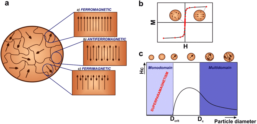
[INSERT DIAGRAM: Ferromagnetic material showing domain structure with arrows indicating magnetization directions in different domains, separated by domain walls

Without an applied field, domains orient randomly to minimize magnetostatic energy. When you apply a field, two processes occur:

Domain wall motion: Favorably oriented domains grow at the expense of others
Domain rotation: Domain magnetizations rotate toward the field direction

The Curie Temperature Transition

Every ferromagnetic material has a critical temperature (Curie temperature, Tᶜ) above which it becomes paramagnetic. This happens because thermal energy overcomes the exchange interaction that maintains domain alignment.

[EQUATION: For T > Tᶜ: χ = C/(T – Tᶜ) – Curie-Weiss Law]

Examples of Curie Temperatures:

Iron: 1043 K (770°C)
Nickel: 631 K (358°C)
Cobalt: 1404 K (1131°C)

Real-World Physics: Curie temperature sensors use this property for temperature measurement and fire detection. When temperature exceeds Tᶜ, ferromagnetic elements lose their magnetism, triggering safety systems.

Soft vs Hard Magnetic Materials

Soft Magnetic Materials (easy to magnetize/demagnetize):

Narrow hysteresis loops
Low coercivity (Hᶜ < 1000 A/m)
Applications: transformer cores, electromagnets, motors

Hard Magnetic Materials (retain magnetization strongly):

Wide hysteresis loops
High coercivity (Hᶜ > 10,000 A/m)
Applications: permanent magnets, magnetic storage media

Section 6: Hysteresis – The Memory of Magnetic Materials

Understanding the Hysteresis Loop

When you cycle a ferromagnetic material through increasing and decreasing magnetic fields, the relationship between magnetic field intensity (H) and magnetic flux density (B) traces a characteristic loop called a hysteresis curve.

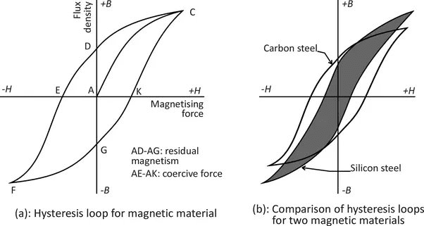
[INSERT DIAGRAM: Complete hysteresis loop showing saturation magnetization, remanence, coercivity, and energy loss area, with clearly labeled axes B vs H

Key Parameters:

Saturation (Bₛₐₜ): Maximum possible magnetization
Remanence/Retentivity (Bᵣ): Residual magnetization when H = 0
Coercivity (Hᶜ): Reverse field needed to reduce B to zero

[EQUATION: Energy dissipated per cycle = ∮ H⋅dB = Area enclosed by hysteresis loop]

Applications Based on Hysteresis Properties

Transformer Cores require materials with narrow hysteresis loops to minimize energy losses during AC operation. Silicon steel is optimized for this application.

Permanent Magnets need wide hysteresis loops with high coercivity to resist demagnetization. Modern neodymium-iron-boron magnets can maintain their magnetization for decades.

Magnetic Storage uses materials where the two directions of remanent magnetization represent binary data (0 and 1).

Problem-Solving Strategy: When analyzing hysteresis problems, always identify whether you’re dealing with soft or hard magnetic materials first. This determines which part of the loop is most important for the application.

Section 7: Earth’s Magnetism – Our Planetary Magnetic Shield

Magnetic Elements and Navigation

Earth behaves like a giant bar magnet with its magnetic axis tilted about 11° from the geographic axis. At any location on Earth, the magnetic field can be completely described by three magnetic elements:

[EQUATION: Total Field Components: B² = Bₕ² + Bᵥ² where Bₕ is horizontal component, Bᵥ is vertical component]

[EQUATION: Magnetic Dip: tan I = Bᵥ/Bₕ where I is the angle of inclination or dip]

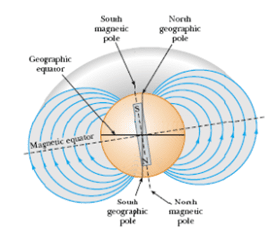
[INSERT DIAGRAM: Earth’s magnetic field lines showing geographic poles, magnetic poles, declination angle, and inclination angle at a specific location

The Three Key Angles

Declination (D): Angle between magnetic north and geographic north
Inclination/Dip (I): Angle between field direction and horizontal plane
Total field magnitude and components

Real-World Physics: GPS systems must constantly update magnetic declination data because Earth’s magnetic field changes over time due to movements in the molten iron core. Declination can vary by several degrees over decades.

Magnetic Maps and Secular Variation

Earth’s magnetic field isn’t constant – it changes slowly over time (secular variation) and occasionally reverses completely. Paleomagnetic studies show that magnetic reversals happen roughly every 200,000 to 300,000 years.

Historical Context: The Chinese discovered magnetic declination over 1000 years ago, noting that compass needles didn’t point to true north. This discovery was crucial for accurate navigation and mapmaking.

Section 8: Laboratory Investigations and Measurement Techniques

Measuring Magnetic Susceptibility – Gouy’s Method

The most common method for measuring magnetic susceptibility uses Gouy’s balance, which measures the apparent change in weight of a sample placed in a non-uniform magnetic field.

[INSERT DIAGRAM: Gouy’s balance setup showing sample tube suspended between electromagnet poles, with sensitive balance measuring weight changes

Experimental Procedure:

Measure sample weight without magnetic field (W₁)
Apply strong non-uniform magnetic field
Measure new apparent weight (W₂)
Calculate susceptibility from weight change

[EQUATION: χ = (2ΔW g)/(ρ A B² μ₀) where ΔW = W₂ – W₁, ρ is density, A is cross-sectional area, g is gravitational acceleration]

Plotting B-H Curves

To obtain hysteresis loops experimentally:

Equipment Needed:

Toroidal core sample with primary and secondary windings
Variable current source for primary coil
Integrating circuit for secondary coil
Oscilloscope or data acquisition system

Key Measurements:

Primary current determines H field
Secondary voltage integration gives B field
Plot B vs H while cycling current

Error Analysis: Account for air gap effects, temperature variations, and eddy current losses in the sample. Proper calibration requires known reference materials.

Determining Curie Temperature

Experimental Design:

Heat ferromagnetic sample gradually while monitoring susceptibility
Note temperature where χ drops sharply (transition to paramagnetic)
Above Tᶜ, verify that susceptibility follows Curie-Weiss law
Use multiple heating/cooling cycles to ensure reproducibility

Section 9: Advanced Applications in Modern Technology

Magnetic Resonance Imaging (MRI)

MRI exploits the magnetic properties of hydrogen nuclei in water molecules. When placed in strong magnetic fields (1-3 Tesla), these nuclear magnetic moments align with the field.

Technical Principle: Radio frequency pulses tip these aligned nuclei, and their relaxation back to equilibrium produces detectable signals. Different tissues have different relaxation times, creating image contrast.

Real-World Physics: MRI machines use superconducting electromagnets cooled with liquid helium to generate ultra-stable magnetic fields. Even tiny field variations would blur images, so magnetic shielding is critical.

Spintronics and Quantum Technology

Modern electronics increasingly exploits electron spin rather than just charge. Spintronic devices like giant magnetoresistance (GMR) sensors revolutionized computer hard drives by dramatically increasing storage density.

Future Applications:

Quantum computers using magnetic quantum dots
Spin-based memory devices (MRAM)
Magnetic logic circuits for ultra-low power electronics

Magnetic Separation and Purification

Industries use magnetic properties for separation processes:

Iron ore processing: Separating magnetic iron minerals from non-magnetic gangue
Recycling: Separating ferrous from non-ferrous metals
Biotechnology: Using magnetic nanoparticles to isolate specific proteins or cells

Section 10: Comprehensive Problem-Solving Guide

Problem Type 1: Magnetic Susceptibility and Permeability Calculations

Sample Problem: A paramagnetic rod has magnetic susceptibility 3.7 × 10⁻⁴. When placed in a magnetic field of 0.8 T, find: (a) relative permeability, (b) magnetization, (c) magnetic field inside the rod.

Step-by-Step Solution:

(a) Relative Permeability:
μᵣ = 1 + χ = 1 + 3.7 × 10⁻⁴ = 1.00037

(b) Magnetization:
First find H: H = B/μ₀ = 0.8/(4π × 10⁻⁷) = 6.37 × 10⁵ A/m
Then: M = χH = 3.7 × 10⁻⁴ × 6.37 × 10⁵ = 235.7 A/m

(c) Magnetic Field Inside:
B_inside = μ₀(H + M) = μ₀H + μ₀M = 0.8 + (4π × 10⁻⁷ × 235.7) = 0.8003 T

Problem Type 2: Earth’s Magnetic Field Elements

Sample Problem: At a location, horizontal component of Earth’s field is 2 × 10⁻⁵ T and dip angle is 45°. Find the total magnetic field and vertical component.

Solution:
Given: Bₕ = 2 × 10⁻⁵ T, I = 45°

Vertical component: Bᵥ = Bₕ tan I = 2 × 10⁻⁵ × tan 45° = 2 × 10⁻⁵ T

Total field: B = Bₕ/cos I = 2 × 10⁻⁵/cos 45° = 2 × 10⁻⁵/0.707 = 2.83 × 10⁻⁵ T

Physics Check: At 45° dip, vertical and horizontal components should be equal, which our answer confirms.

Problem Type 3: Hysteresis and Energy Loss

Sample Problem: A ferromagnetic core operates in an AC magnetic field. If the hysteresis loop has area 200 J/m³ per cycle and the core volume is 0.01 m³, find energy dissipated per second at 50 Hz.

Solution:
Energy per cycle = Area × Volume = 200 × 0.01 = 2 J/cycle
Power = Energy per cycle × Frequency = 2 × 50 = 100 W

Problem Type 4: Temperature Effects on Magnetic Properties

Sample Problem: A paramagnetic material follows Curie’s law with C = 0.8 K. Find the ratio of susceptibilities at 300 K and 600 K.

Solution:
χ₁/χ₂ = (C/T₁)/(C/T₂) = T₂/T₁ = 600/300 = 2

The susceptibility at 300 K is twice that at 600 K, showing how thermal motion reduces magnetic alignment.

Section 11: Practice Problems Collection

Multiple Choice Questions with Detailed Solutions

Q1: Which material would show the strongest diamagnetic response?
(a) Copper (b) Bismuth (c) Aluminum (d) Iron

Answer: (b) Bismuth
Detailed Explanation: Bismuth has χ = -1.66 × 10⁻⁴, the strongest diamagnetic response among common elements. Copper is also diamagnetic but weaker (χ ≈ -10⁻⁵). Aluminum is paramagnetic, and iron is ferromagnetic.

Q2: The magnetic susceptibility of a material is -0.5 × 10⁻⁵. The material is:
(a) Ferromagnetic (b) Paramagnetic (c) Diamagnetic (d) Cannot be determined

Answer: (c) Diamagnetic
Detailed Explanation: Negative susceptibility is the defining characteristic of diamagnetic materials. The magnitude (10⁻⁵) is typical for diamagnetic substances.

Q3: At the magnetic equator, Earth’s magnetic field:
(a) Is purely horizontal (b) Is purely vertical (c) Has equal horizontal and vertical components (d) Is zero

Answer: (a) Is purely horizontal
Detailed Explanation: At the magnetic equator, the dip angle I = 0°, so Bᵥ = Bₕ tan 0° = 0. The field is entirely horizontal.

Free Response Problems with Complete Solutions

Problem 1: A toroidal electromagnet has a ferromagnetic core with relative permeability 2000. The electromagnet has 500 turns carrying 2 A current. If the mean path length through the core is 0.3 m, find:
(a) Magnetic field intensity H in the core
(b) Magnetic flux density B in the core
(c) Magnetization M of the core material

Complete Solution:

(a) Magnetic Field Intensity:
Using Ampère’s law for toroidal geometry:
H = NI/(2πr_avg) ≈ NI/l_path = (500 × 2)/0.3 = 3333 A/m

(b) Magnetic Flux Density:
B = μ₀μᵣH = 4π × 10⁻⁷ × 2000 × 3333 = 8.38 T

(c) Magnetization:
M = χH = (μᵣ – 1)H = (2000 – 1) × 3333 = 6.66 × 10⁶ A/m

Problem 2: Design an experiment to distinguish between paramagnetic and diamagnetic liquids using simple laboratory equipment.

Experimental Design:

Objective: Differentiate paramagnetic from diamagnetic liquids

Materials: Strong permanent magnet, glass tubes, various liquid samples, sensitive balance or visual observation setup

Procedure:

Fill identical glass tubes with test liquids
Suspend tubes horizontally near magnet pole
Observe deflection direction:

Paramagnetic liquids: Attracted toward magnet
Diamagnetic liquids: Repelled from magnet

Controls: Test known paramagnetic (liquid oxygen, if available) and diamagnetic (water) samples first

Quantitative Enhancement: Use Gouy balance method to measure actual susceptibility values

Safety: Ensure strong magnets don’t interfere with electronic devices; handle glass tubes carefully

Section 12: Exam Success Strategies and Common Pitfalls

High-Frequency Exam Topics

Based on CBSE exam patterns, these topics appear most frequently:

Classification of magnetic materials (40% of questions)
Magnetic susceptibility calculations (25% of questions)
Earth’s magnetic elements (20% of questions)
Curie temperature and temperature effects (10% of questions)
Hysteresis applications (5% of questions)

Common Mistakes and Prevention Strategies

Mistake 1: Confusing signs of magnetic susceptibility
Prevention: Remember “DPF” – Diamagnetic (negative), Paramagnetic (positive small), Ferromagnetic (positive large)

Mistake 2: Incorrect unit conversions between B and H
Prevention: Always write B = μ₀H in vacuum, B = μ₀μᵣH in materials

Mistake 3: Misinterpreting hysteresis loop parameters
Prevention: Practice sketching loops and identifying remanence, coercivity, and saturation points

Mistake 4: Wrong application of Curie’s law
Prevention: Remember Curie’s law applies only to paramagnetic materials above their Curie temperature

Time Management for Different Question Types

2-mark questions (Definition/Classification): 2-3 minutes each

Focus on clear definitions and examples
Use proper scientific terminology

3-mark questions (Numerical problems): 4-5 minutes each

Show all steps clearly
Include proper units throughout
State final answer explicitly

5-mark questions (Derivations/Applications): 8-10 minutes each

Start with basic principles
Show mathematical steps logically
Connect to real-world applications

Conclusion: Mastering Magnetism for Academic and Career Success

Congratulations! You’ve journeyed through the fascinating world of magnetism and matter, from atomic magnetic moments to Earth’s protective magnetic shield. This chapter isn’t just about passing exams – it’s your introduction to understanding the magnetic technologies that power our modern world.

Every time you use magnetic storage, navigate with GPS, get an MRI scan, or even stick a note to your refrigerator, you’re witnessing the principles you’ve mastered here. The classification skills you’ve developed help engineers choose materials for everything from transformer cores to permanent magnets in electric vehicles.

Key Conceptual Takeaways:

All materials respond to magnetic fields, but in distinctly different ways based on their atomic structure
Temperature plays a crucial role in magnetic behavior, with thermal energy competing against magnetic alignment
Ferromagnetic materials’ ability to maintain magnetization makes most magnetic technology possible
Earth’s magnetic field, while seemingly simple, involves complex three-dimensional field geometry

Mathematical Mastery Achieved:
You can now calculate magnetic susceptibility, permeability, and field strengths in different materials. You understand the temperature dependencies described by Curie’s law and can analyze hysteresis loops to determine energy losses in magnetic systems.

Problem-Solving Skills Developed:
Your systematic approach to magnetism problems – identifying material type, choosing appropriate equations, and checking answer reasonableness – will serve you well in engineering and physics courses ahead.

Real-World Connections:
From MRI machines using superconducting magnets to the magnetic separation processes in recycling facilities, you can now appreciate the physics behind technologies that improve our lives daily.

Future Learning Pathways:
This foundation prepares you for advanced topics in electromagnetism, quantum mechanics, and materials science. In university physics and engineering courses, you’ll explore quantum origins of magnetism, advanced magnetic materials, and cutting-edge applications in quantum computing and spintronics.

Final Exam Strategy:
Remember that magnetism problems often connect to other physics topics. Don’t just memorize formulas – understand the underlying physics so you can adapt to novel problem scenarios in your board exam.

As you continue your physics journey, carry with you the wonder that motivated scientists like Curie, Faraday, and Maxwell. The magnetic phenomena you’ve studied here continue to reveal new secrets, from magnetic monopoles in exotic materials to the magnetic fields of distant galaxies.

The invisible magnetic forces you now understand are among the fundamental interactions that shaped our universe and continue to drive technological innovation. Your mastery of these concepts opens doors to careers in physics, engineering, medicine, and emerging fields we can barely imagine today.

Good luck with your CBSE board examination! Your deep understanding of magnetism and matter will serve you well not just in scoring excellent marks, but in appreciating the magnetic world around you for years to come.

This comprehensive study guide provides everything needed to excel in CBSE Class 12 Physics Chapter 5. Continue practicing problems, connecting concepts to real-world phenomena, and maintaining curiosity about the magnetic forces that surround us every day.

Recommended –