

Introduction: Welcome to the Quantum World Around You
Every time you use your smartphone, scan a barcode at the grocery store, or see the glow of an LED light, you’re witnessing Modern Physics in action. The quantum world isn’t just a theoretical playground for physicists-it’s the foundation of virtually every piece of technology you interact with daily. From the GPS satellites that guide your navigation apps (which must account for relativistic effects) to the solar panels powering homes worldwide (based on the photoelectric effect), modern physics governs the invisible mechanisms that shape our contemporary world.
Unit 15 of AP Physics 2 takes you on an extraordinary journey from the classical physics you’ve mastered into the counterintuitive realm of quantum mechanics, atomic structure, and nuclear physics. You’ll discover why particles sometimes behave like waves, how energy comes in discrete packets called quanta, and why atoms are simultaneously incredibly stable and capable of releasing enormous amounts of energy.
This isn’t just about memorizing equations and solving problems-though you’ll do plenty of both. Modern physics represents humanity’s greatest intellectual achievement: understanding the fundamental nature of matter, energy, space, and time. When you grasp these concepts, you’re thinking the same thoughts that revolutionized science in the early 20th century and continue to drive technological innovation today.
Whether you’re planning a career in engineering, medicine, computer science, or pure research, the principles you’ll learn in this unit form the bedrock of cutting-edge fields like quantum computing, medical imaging, renewable energy, and space exploration. More immediately, mastering Unit 15 is crucial for AP exam success, as modern physics problems often integrate concepts from throughout the course and require sophisticated problem-solving skills.
Learning Objectives: Your Roadmap to Modern Physics Mastery
By the end of this comprehensive study guide, you’ll have developed a deep understanding of modern physics that aligns perfectly with College Board AP Physics 2 standards. Your learning journey will encompass both conceptual mastery and practical problem-solving skills:
Quantum Mechanics and Wave-Particle Duality: You’ll explain how electromagnetic radiation and matter exhibit both wave and particle properties, analyze photon energy and momentum relationships, and solve problems involving the de Broglie wavelength. You’ll understand why classical physics fails at atomic scales and how quantum mechanics provides accurate predictions.
Photoelectric Effect and Photon Interactions: You’ll master Einstein’s photon theory, calculate maximum kinetic energies of photoelectrons, analyze stopping potential graphs, and explain why the photoelectric effect cannot be explained by classical wave theory. You’ll connect these concepts to modern applications like photovoltaic cells and photomultiplier tubes.
Atomic Structure and Energy Levels: You’ll model atomic structure using quantum mechanical principles, calculate energy level transitions, analyze emission and absorption spectra, and explain how atoms achieve stability. You’ll understand electron configurations, orbital models, and the relationship between atomic structure and chemical properties.
Nuclear Physics and Radioactivity: You’ll analyze nuclear reactions, calculate binding energies, understand radioactive decay processes, and apply conservation laws to nuclear interactions. You’ll explore both the beneficial applications of nuclear physics (medical imaging, power generation) and associated safety considerations.
Mass-Energy Equivalence: You’ll apply Einstein’s famous equation E = mc² to calculate energy released in nuclear reactions, understand the source of stellar energy, and analyze particle creation and annihilation processes. You’ll connect mass-energy equivalence to nuclear binding energy and stability.
Experimental Design and Data Analysis: You’ll design experiments to investigate modern physics phenomena, analyze data from photelectric effect measurements, interpret spectroscopic data, and evaluate experimental uncertainties. You’ll understand how key historical experiments led to our current understanding of atomic and nuclear structure.
1: The Quantum Revolution – From Classical to Modern Physics
The transition from classical to modern physics represents one of the most dramatic paradigm shifts in scientific history. Understanding this transition is crucial because it explains why the familiar laws of Newton, Maxwell, and thermodynamics that you’ve studied throughout AP Physics suddenly seem inadequate when dealing with atomic-scale phenomena.
Classical physics, developed over centuries by brilliant minds like Newton, Maxwell, and Boltzmann, successfully describes the motion of planets, the behavior of electromagnetic waves, and the properties of gases. However, by the late 1800s, several experimental observations stubbornly refused to conform to classical predictions. These “failures” of classical physics weren’t minor discrepancies-they were fundamental contradictions that demanded entirely new theoretical frameworks.
The Ultraviolet Catastrophe and Blackbody Radiation
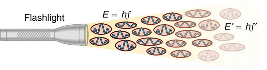
Consider a simple scenario: heating a piece of metal until it glows. Classical physics predicted that hot objects should emit infinite amounts of ultraviolet radiation, clearly contradicting everyday experience. This “ultraviolet catastrophe” was resolved when Max Planck proposed in 1900 that energy could only be emitted in discrete packets, or quanta, with energy E = hf, where h is Planck’s constant and f is frequency.
[EQUATION: Planck’s Energy Quantization: E = hf = hc/λ, where h = 6.626 × 10⁻³⁴ J·s is Planck’s constant, f is frequency in Hz, c = 3.00 × 10⁸ m/s is the speed of light, and λ is wavelength in meters]
This seemingly simple equation revolutionized physics by introducing the concept of energy quantization. Energy wasn’t continuous, as classical physics assumed, but came in discrete chunks proportional to frequency. Higher frequency radiation (blue light, ultraviolet, X-rays) carries more energy per photon than lower frequency radiation (red light, infrared, radio waves).
Wave-Particle Duality: The Heart of Quantum Mechanics
Perhaps the most mind-bending aspect of modern physics is wave-particle duality-the idea that both electromagnetic radiation and matter exhibit properties of both waves and particles, depending on how they’re observed. This isn’t simply a matter of our measurement techniques being imperfect; it’s a fundamental property of nature at quantum scales.
For electromagnetic radiation, this duality manifests in phenomena like the photoelectric effect, where light behaves as discrete particles (photons), and interference patterns, where light clearly behaves as waves. The key insight is that particle and wave descriptions aren’t contradictory but complementary-different aspects of a more complete quantum mechanical description.
Real-World Physics: Quantum Effects in Everyday Technology
Your smartphone’s camera relies on the photoelectric effect to convert light into electrical signals. LED lights work because electrons transition between discrete energy levels in semiconductor materials. Laser pointers produce coherent light through stimulated emission, a purely quantum mechanical process. Even the stability of atoms themselves depends on quantum mechanics-without electron wave functions and the Pauli exclusion principle, matter as we know it couldn’t exist.
Common Error Alert: Mixing Classical and Quantum Concepts
Students often struggle when trying to apply classical intuition to quantum phenomena. Remember that at atomic scales, particles don’t have definite positions and velocities simultaneously (Heisenberg uncertainty principle), energy levels are discrete rather than continuous, and observation itself affects the system being measured. When solving modern physics problems, always check whether classical concepts like “trajectory” or “exact position” are even meaningful in the given context.
2: Photons and the Photoelectric Effect – Light as Particles
The photoelectric effect stands as one of the most elegant demonstrations of light’s particle nature and earned Albert Einstein the 1921 Nobel Prize in Physics. Understanding this phenomenon deeply will give you powerful tools for analyzing how light interacts with matter and provide a foundation for more advanced quantum mechanical concepts.
Einstein’s Revolutionary Photon Theory
When Einstein analyzed the photoelectric effect in 1905, he proposed that electromagnetic radiation consists of discrete energy packets called photons. Each photon carries energy E = hf and momentum p = h/λ = hf/c. This particle description of light explained experimental observations that classical wave theory could not.
[EQUATION: Photoelectric Effect Energy Conservation: hf = KEmax + φ, where hf is the incident photon energy, KEmax is the maximum kinetic energy of emitted photoelectrons, and φ is the work function of the material]
The work function φ represents the minimum energy required to remove an electron from the material’s surface. It’s a characteristic property of each material, typically measured in electron volts (eV), where 1 eV = 1.602 × 10⁻¹⁹ J.
Key Experimental Observations
The photoelectric effect exhibits several counterintuitive features that classical physics cannot explain:
Threshold Frequency: Below a certain frequency f₀ = φ/h, no photoelectrons are emitted regardless of light intensity. This threshold frequency is different for each material and depends only on the work function.
Instantaneous Emission: Photoelectrons are emitted immediately when light above the threshold frequency strikes the surface, even at very low intensities. Classical wave theory predicted a time delay for low-intensity light.
Independence from Intensity: The maximum kinetic energy of photoelectrons depends only on frequency, not intensity. Increasing intensity increases the number of photoelectrons but not their individual energies.
Linear Relationship: A graph of KEmax versus frequency yields a straight line with slope h and y-intercept -φ. This linear relationship provided one of the first accurate measurements of Planck’s constant.
Stopping Potential Analysis
In photoelectric effect experiments, the stopping potential V₀ is the minimum voltage needed to prevent photoelectrons from reaching a collector. The relationship between stopping potential and maximum kinetic energy is:
[EQUATION: Stopping Potential: eV₀ = KEmax = hf – φ, where e = 1.602 × 10⁻¹⁹ C is the elementary charge]
Problem-Solving Strategy: Photoelectric Effect Problems
- Identify given information: frequency or wavelength of incident light, work function of material, stopping potential, or kinetic energy of photoelectrons
- Determine what to find: often maximum kinetic energy, threshold frequency, or stopping potential
- Choose appropriate equation: Use hf = KEmax + φ for energy conservation, or eV₀ = KEmax for stopping potential problems
- Convert units consistently: Ensure energy units match (Joules or eV), convert wavelength to frequency if needed using c = fλ
- Check reasonableness: Maximum kinetic energy should be positive, threshold frequency should make physical sense for the given material
Worked Example: Cesium Photoelectric Effect
Light with wavelength 400 nm strikes a cesium surface (work function φ = 2.1 eV). Calculate the maximum kinetic energy of emitted photoelectrons and the stopping potential.
Step 1: Convert wavelength to frequency
f = c/λ = (3.00 × 10⁸ m/s)/(400 × 10⁻⁹ m) = 7.50 × 10¹⁴ Hz
Step 2: Calculate photon energy
E = hf = (6.626 × 10⁻³⁴ J·s)(7.50 × 10¹⁴ Hz) = 4.97 × 10⁻¹⁹ J
Converting to eV: E = (4.97 × 10⁻¹⁹ J)/(1.602 × 10⁻¹⁹ J/eV) = 3.10 eV
Step 3: Apply energy conservation
KEmax = hf – φ = 3.10 eV – 2.1 eV = 1.0 eV
Step 4: Calculate stopping potential
V₀ = KEmax/e = 1.0 eV/e = 1.0 V
Physics Check: Understanding Photon Momentum
Although photons have zero rest mass, they carry momentum p = E/c = hf/c = h/λ. This momentum is crucial in phenomena like radiation pressure and Compton scattering. When a photon strikes an electron, both energy and momentum must be conserved, leading to the Compton effect where the scattered photon has lower energy and longer wavelength than the incident photon.
3: Atomic Structure and Energy Levels – The Quantum Atom
The development of atomic models represents a fascinating journey from simple “plum pudding” models to sophisticated quantum mechanical descriptions. Understanding atomic structure is essential not only for AP Physics 2 success but also for comprehending how the entire periodic table organizes, why chemical bonds form, and how atoms emit and absorb light.
From Rutherford to Bohr: Building the Nuclear Atom
Ernest Rutherford’s famous gold foil experiment in 1909 revealed that atoms consist mostly of empty space with a tiny, dense nucleus containing all the positive charge and most of the mass. However, this nuclear model created a serious problem: according to classical physics, orbiting electrons should continuously radiate electromagnetic energy and spiral into the nucleus in about 10⁻¹⁰ seconds. Obviously, this doesn’t happen, since atoms are stable.
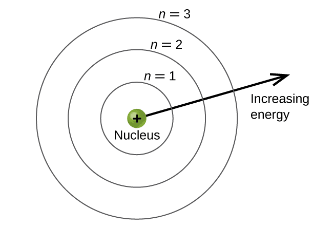
Niels Bohr solved this crisis in 1913 by proposing that electrons occupy only certain allowed orbits with quantized angular momentum. In these special orbits, electrons don’t radiate energy despite being accelerated. Only when electrons transition between orbits do they emit or absorb photons with energy equal to the difference between energy levels.
The Bohr Model and Hydrogen Energy Levels
The Bohr model provides an excellent introduction to quantum concepts and works remarkably well for hydrogen atoms. The key assumptions are:
- Electrons orbit the nucleus in circular paths with quantized angular momentum: L = nℏ, where n is a positive integer and ℏ = h/2π
- Electrons in allowed orbits don’t radiate electromagnetic energy
- Photons are emitted or absorbed when electrons transition between orbits
[EQUATION: Hydrogen Energy Levels: En = -13.6 eV/n², where n = 1, 2, 3, … is the principal quantum number]
The negative energy values indicate that electrons are bound to the nucleus. The n = 1 level (ground state) has the lowest energy at -13.6 eV, while higher levels have less negative (higher) energies, approaching zero as n approaches infinity.
Atomic Transitions and Spectroscopy
When an electron transitions from a higher energy level (ni) to a lower energy level (nf), it emits a photon with energy:
[EQUATION: Photon Energy in Atomic Transitions: Ephoton = Ei – Ef = 13.6 eV(1/nf² – 1/ni²)]
The frequency and wavelength of this photon are related by E = hf = hc/λ, allowing us to calculate the exact wavelength of emitted light.
Spectroscopic Series in Hydrogen
Different series of spectral lines correspond to transitions ending at different levels:
- Lyman series: Transitions to n = 1 (ultraviolet region)
- Balmer series: Transitions to n = 2 (visible region)
- Paschen series: Transitions to n = 3 (infrared region)
The most famous line in the Balmer series is the red Hα line (n = 3 → n = 2), which gives hydrogen gas its characteristic red glow and is prominent in astronomical observations.
Real-World Physics: Applications of Atomic Spectroscopy
Atomic spectroscopy is far more than a theoretical curiosity. Astronomers use spectral lines to determine the composition of distant stars and galaxies. Medical imaging techniques like MRI rely on nuclear magnetic resonance, a quantum mechanical phenomenon. Atomic clocks, which provide the time standard for GPS satellites, depend on precise atomic transitions in cesium or rubidium atoms.
Beyond Bohr: Quantum Mechanical Improvements
While the Bohr model successfully explains hydrogen spectra, it fails for multi-electron atoms and doesn’t account for fine structure in spectral lines. The complete quantum mechanical treatment introduces additional quantum numbers:
- Principal quantum number (n): Determines energy level (1, 2, 3, …)
- Orbital angular momentum (ℓ): Determines orbital shape (0, 1, 2, …, n-1)
- Magnetic quantum number (mℓ): Determines orbital orientation (-ℓ, …, 0, …, +ℓ)
- Spin quantum number (ms): Determines electron spin (±1/2)
Problem-Solving Strategy: Atomic Energy Level Problems
- Identify the transition: Determine initial and final quantum numbers (ni and nf)
- Calculate energy difference: Use ΔE = 13.6 eV(1/nf² – 1/ni²) for hydrogen
- Determine photon properties: Use E = hf = hc/λ to find frequency or wavelength
- Check energy conservation: Energy is conserved in all atomic processes
- Consider direction: Emission involves ni > nf, absorption involves ni < nf
Worked Example: Balmer Series Calculation
Calculate the wavelength of light emitted when a hydrogen electron transitions from n = 4 to n = 2.
Step 1: Calculate energy difference
ΔE = 13.6 eV(1/2² – 1/4²) = 13.6 eV(1/4 – 1/16) = 13.6 eV(3/16) = 2.55 eV
Step 2: Convert to Joules
ΔE = 2.55 eV × 1.602 × 10⁻¹⁹ J/eV = 4.09 × 10⁻¹⁹ J
Step 3: Calculate wavelength
λ = hc/E = (6.626 × 10⁻³⁴ J·s)(3.00 × 10⁸ m/s)/(4.09 × 10⁻¹⁹ J) = 486 nm
This blue-green light is indeed observed in hydrogen emission spectra and is known as the Hβ line.
4: De Broglie Wavelength and Matter Waves
One of the most revolutionary concepts in modern physics is the idea that matter, like electromagnetic radiation, exhibits wave properties. This concept, introduced by Louis de Broglie in 1924, extended wave-particle duality from photons to all matter and laid the groundwork for quantum mechanics as we know it today.
De Broglie’s Hypothesis
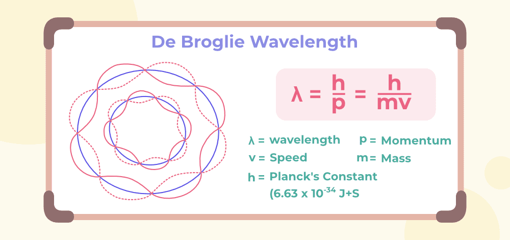
De Broglie proposed that any particle with momentum p has an associated wavelength λ given by:
[EQUATION: De Broglie Wavelength: λ = h/p = h/(mv), where h is Planck’s constant, p is momentum, m is mass, and v is velocity]
This relationship applies to all matter, from electrons and protons to baseballs and planets. However, the wave nature becomes observable only when the de Broglie wavelength is comparable to the size of the system or obstacles the particle encounters.
Why Don’t We Notice Matter Waves in Daily Life?
Consider a 0.1 kg baseball moving at 30 m/s. Its de Broglie wavelength is:
λ = h/(mv) = (6.626 × 10⁻³⁴ J·s)/[(0.1 kg)(30 m/s)] = 2.2 × 10⁻³⁴ m
This wavelength is incredibly tiny-much smaller than atoms, nuclei, or even elementary particles. Since there are no structures small enough to interact with such short wavelengths, the baseball’s wave nature is completely unobservable.
Electron Wave Properties
For electrons, the situation is dramatically different. An electron moving at 10⁶ m/s has a de Broglie wavelength of:
λ = h/(mv) = (6.626 × 10⁻³⁴ J·s)/[(9.109 × 10⁻³¹ kg)(10⁶ m/s)] = 7.3 × 10⁻¹⁰ m
This wavelength is comparable to atomic dimensions, making electron wave properties readily observable in phenomena like electron diffraction and the stability of atomic orbitals.
Experimental Confirmation: Electron Diffraction
The wave nature of electrons was dramatically confirmed in 1927 by Clinton Davisson and Lester Germer, who observed diffraction patterns when electrons scattered from a nickel crystal. These experiments showed that electrons behave exactly like X-rays when interacting with crystal structures, producing constructive and destructive interference patterns.
Quantum Mechanical Implications
De Broglie’s matter waves led directly to Schrödinger’s wave equation, the fundamental equation of quantum mechanics. The wave function ψ describes the probability amplitude of finding a particle at different locations, with |ψ|² giving the probability density.
This probabilistic interpretation resolves the mystery of atomic stability. Electrons in atoms aren’t “orbiting” in the classical sense but exist as standing wave patterns around the nucleus. Only certain wavelengths can form stable standing waves, naturally explaining energy level quantization without arbitrary assumptions.
Standing Waves in Atoms
For an electron in a circular orbit to form a stable standing wave, the orbit circumference must be an integer multiple of the de Broglie wavelength:
[EQUATION: Bohr-de Broglie Condition: 2πr = nλ = nh/(mv), which leads to mvr = nℏ]
This naturally derives Bohr’s quantization condition from wave mechanics, showing that the Bohr model emerges as a classical limit of quantum mechanics.
Problem-Solving Strategy: De Broglie Wavelength Problems
- Identify given information: mass, velocity, kinetic energy, or momentum of the particle
- Calculate momentum: Use p = mv for non-relativistic particles, or p = √(2mKE) if given kinetic energy
- Apply de Broglie relation: λ = h/p
- Check units: Ensure wavelength comes out in meters
- Assess observability: Compare wavelength to relevant physical dimensions
Worked Example: Electron Microscopy
Electrons in an electron microscope are accelerated through a potential difference of 50 kV. Calculate their de Broglie wavelength and explain why electron microscopes achieve better resolution than optical microscopes.
Step 1: Calculate electron kinetic energy
KE = eV = (1.602 × 10⁻¹⁹ C)(50,000 V) = 8.01 × 10⁻¹⁵ J
Step 2: Calculate momentum (non-relativistic approximation)
p = √(2mKE) = √(2 × 9.109 × 10⁻³¹ kg × 8.01 × 10⁻¹⁵ J) = 1.21 × 10⁻²² kg⋅m/s
Step 3: Calculate de Broglie wavelength
λ = h/p = (6.626 × 10⁻³⁴ J⋅s)/(1.21 × 10⁻²² kg⋅m/s) = 5.48 × 10⁻¹² m = 5.48 pm
Step 4: Compare to visible light
Visible light wavelengths range from about 400-700 nm, while these electrons have a wavelength of only 5.48 pm-about 100,000 times shorter. Since resolution is limited by wavelength, electron microscopes can resolve features much smaller than those visible with optical microscopes.
Physics Check: Relativistic Considerations
For very high-energy electrons, relativistic effects become important. The total energy is E = γmc², where γ is the Lorentz factor, and momentum is p = γmv. Always check whether relativistic corrections are needed by comparing the kinetic energy to the rest energy (mc² = 0.511 MeV for electrons).
5: Nuclear Physics – The Heart of the Atom
Nuclear physics opens the door to understanding both the most fundamental building blocks of matter and some of the most powerful phenomena in the universe. From the fusion reactions that power stars to the medical isotopes that save lives, nuclear processes shape our world in ways both dramatic and subtle.
Nuclear Structure and Composition
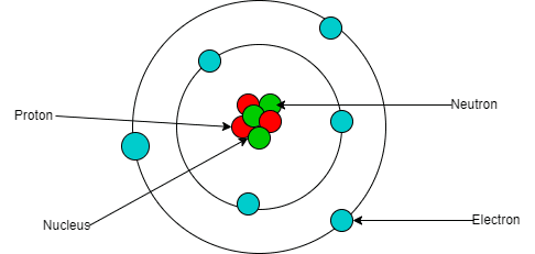
Atomic nuclei consist of protons and neutrons (collectively called nucleons) held together by the strong nuclear force. The number of protons (Z) defines the element, while the total number of nucleons (A) gives the mass number. Isotopes of an element have the same Z but different numbers of neutrons.
Nuclear notation typically appears as ᴬZX, where X is the chemical symbol. For example, ²³⁸U₉₂ represents uranium-238 with 238 total nucleons and 92 protons (thus 146 neutrons).
The Strong Nuclear Force
The strong nuclear force is fundamentally different from electromagnetic and gravitational forces. It’s extremely powerful but has a very short range (about 10⁻¹⁵ m). This force binds protons and neutrons together despite the electromagnetic repulsion between positively charged protons.
Nuclear Binding Energy
Perhaps the most important concept in nuclear physics is binding energy-the energy required to completely separate a nucleus into individual nucleons. This energy manifests as a mass defect: the mass of a nucleus is always less than the sum of its constituent nucleons’ masses.
[EQUATION: Mass-Energy Equivalence: E = mc², where c = 2.998 × 10⁸ m/s]
[EQUATION: Binding Energy: BE = (Zmₚ + Nmₙ – M)c², where mₚ is proton mass, mₙ is neutron mass, M is nuclear mass, and N = A – Z is the number of neutrons]
Atomic Mass Units and Conversion
Nuclear physics calculations are simplified using atomic mass units (u), where 1 u = 931.5 MeV/c². Key masses to remember:
- Proton: mₚ = 1.007276 u
- Neutron: mₙ = 1.008665 u
- Electron: mₑ = 0.000549 u
Nuclear Stability and the Valley of Stability
Not all combinations of protons and neutrons form stable nuclei. The valley of stability represents the narrow band of N/Z ratios that produce stable isotopes. Nuclei with too many or too few neutrons undergo radioactive decay to reach more stable configurations.
Light nuclei (Z < 20) are most stable when N ≈ Z. Heavier nuclei require more neutrons than protons for stability due to increasing electromagnetic repulsion among protons.
Radioactive Decay Processes
Unstable nuclei achieve stability through several decay modes:
Alpha Decay: Emission of an alpha particle (⁴He₂ nucleus)
ᴬZX → ᴬ⁻⁴Z₋₂Y + ⁴He₂
Beta-minus Decay: A neutron converts to a proton, electron, and antineutrino
ᴬZX → ᴬZ₊₁Y + e⁻ + ν̄ₑ
Beta-plus Decay: A proton converts to a neutron, positron, and neutrino
ᴬZX → ᴬZ₋₁Y + e⁺ + νₑ
Gamma Decay: Emission of high-energy photons from excited nuclear states
ᴬZX* → ᴬZX + γ
Radioactive Decay Law
Radioactive decay follows exponential behavior described by:
[EQUATION: Decay Law: N(t) = N₀e⁻λt, where N(t) is the number of nuclei at time t, N₀ is the initial number, and λ is the decay constant]
[EQUATION: Half-life: t₁/₂ = ln(2)/λ = 0.693/λ]
Conservation Laws in Nuclear Reactions
All nuclear reactions must conserve:
- Mass-energy: Total relativistic energy is conserved
- Charge: Total electric charge is conserved
- Mass number: Total number of nucleons is conserved
- Momentum: Total momentum is conserved
Problem-Solving Strategy: Nuclear Physics Problems
- Identify the process: Determine whether you’re dealing with decay, fusion, fission, or another nuclear reaction
- Apply conservation laws: Use conservation of mass number, charge, and energy
- Calculate Q-values: For reactions, Q = (initial masses – final masses)c²
- Handle decay problems: Use exponential decay equations for half-life problems
- Check reasonableness: Energy values should be in MeV range for nuclear processes
Worked Example: Alpha Decay of Radium-226
Radium-226 undergoes alpha decay. Write the complete reaction equation and calculate the Q-value given: ²²⁶Ra mass = 226.025 u, ²²²Rn mass = 222.018 u, ⁴He mass = 4.003 u.
Step 1: Write the decay equation
²²⁶Ra₈₈ → ²²²Rn₈₆ + ⁴He₂
Step 2: Verify conservation laws
Mass number: 226 = 222 + 4 ✓
Charge: 88 = 86 + 2 ✓
Step 3: Calculate Q-value
Q = (initial mass – final masses)c²
Q = (226.025 – 222.018 – 4.003) u × 931.5 MeV/u
Q = (0.004 u) × 931.5 MeV/u = 3.73 MeV
This positive Q-value indicates the reaction is energetically favorable (exothermic).
Real-World Physics: Nuclear Applications
Nuclear physics powers both beneficial technologies and concerning weapons. Nuclear reactors generate electricity through controlled fission reactions. Medical radioisotopes enable cancer treatment and diagnostic imaging. Carbon-14 dating allows archaeologists to determine the age of organic artifacts. Nuclear magnetic resonance (NMR) provides detailed images of soft tissues in medical applications.
Common Error Alert: Mass-Energy Calculations
Students often confuse atomic masses with nuclear masses. Atomic masses include electron masses, so be careful when calculating nuclear binding energies. Also, remember that binding energy is the energy required to disassemble a nucleus-it’s released when the nucleus forms, making it negative in some energy accounting systems.
6: Nuclear Reactions and Applications
Nuclear reactions represent some of the most energetic processes accessible to human technology. Understanding these reactions is crucial not only for mastering AP Physics 2 concepts but also for appreciating how nuclear science impacts medicine, energy production, and our understanding of stellar processes.
Types of Nuclear Reactions
Nuclear reactions differ fundamentally from chemical reactions because they involve changes in nuclear composition rather than electron arrangements. The enormous energy scales (MeV vs. eV) reflect the strength of nuclear forces compared to electromagnetic forces.
Nuclear Fusion
Fusion reactions combine light nuclei to form heavier nuclei, releasing energy because the products have higher binding energy per nucleon. The most important fusion reactions occur in stellar cores:
Proton-proton chain: 4¹H₁ → ⁴He₂ + 2e⁺ + 2νₑ + 26.7 MeV
This reaction powers our Sun, converting about 600 million tons of hydrogen into helium every second. The mass defect of 0.7% becomes pure energy according to E = mc².
Nuclear Fission
Fission reactions split heavy nuclei into lighter fragments, releasing energy because heavy nuclei have lower binding energy per nucleon than medium-mass nuclei. A typical uranium-235 fission reaction:
²³⁵U + n → ¹⁴¹Ba + ⁹²Kr + 3n + 200 MeV
The released neutrons can trigger additional fission reactions, creating a chain reaction. Controlling this chain reaction enables nuclear power generation, while uncontrolled reactions produce nuclear weapons.
Calculating Reaction Energies (Q-values)
The energy released in nuclear reactions comes from mass differences between reactants and products:
[EQUATION: Q-value: Q = (Σminitial – Σmfinal)c² = Δmc²]
Positive Q-values indicate exothermic reactions that release energy, while negative Q-values require energy input (endothermic reactions).
Threshold Energy for Nuclear Reactions
For endothermic reactions, there’s a minimum kinetic energy (threshold energy) required to make the reaction proceed. This threshold energy is always greater than |Q| due to conservation of momentum:
[EQUATION: Threshold Energy: KEth = -Q(1 + mprojectile/mtarget + mprojectile/mproduct)]
Worked Example: Deuteron-Tritium Fusion
Calculate the Q-value for the fusion reaction: ²H + ³H → ⁴He + n
Given masses: ²H = 2.014 u, ³H = 3.016 u, ⁴He = 4.003 u, n = 1.009 u
Step 1: Calculate initial and final masses
Initial: 2.014 + 3.016 = 5.030 u
Final: 4.003 + 1.009 = 5.012 u
Step 2: Calculate mass defect
Δm = 5.030 – 5.012 = 0.018 u
Step 3: Convert to energy
Q = Δmc² = 0.018 u × 931.5 MeV/u = 16.8 MeV
This large energy release makes deuterium-tritium fusion attractive for power generation, though the technical challenges remain formidable.
Nuclear Power Generation
Nuclear reactors use controlled fission to generate electricity. The key components include:
Fuel: Enriched uranium (3-5% ²³⁵U) formed into pellets and fuel rods
Moderator: Water or graphite that slows neutrons to thermal energies where fission is most probable
Control rods: Neutron-absorbing materials (cadmium, boron) that regulate the chain reaction
Coolant: Removes heat from the reactor core to generate steam for electricity production
The multiplication factor k determines reactor behavior:
- k < 1: Subcritical (reaction dies out)
- k = 1: Critical (steady-state operation)
- k > 1: Supercritical (increasing reaction rate)
Medical Applications of Nuclear Physics
Nuclear medicine uses radioactive isotopes for both diagnosis and treatment:
Diagnostic Imaging: Technetium-99m (t₁/₂ = 6 hours) is ideal for medical imaging because it emits gamma rays for detection but decays quickly to minimize radiation exposure.
Cancer Treatment: Cobalt-60 and cesium-137 provide intense gamma radiation for external beam therapy, while radioactive seeds can be implanted directly in tumors.
Positron Emission Tomography (PET): Uses positron-emitting isotopes like fluorine-18. When positrons annihilate with electrons, they produce characteristic 511-keV gamma rays detected by the scanner.
Carbon Dating
Carbon-14 dating exemplifies nuclear physics applications in archaeology and geology. Living organisms maintain a constant ¹⁴C/¹²C ratio by exchanging carbon with the atmosphere. After death, ¹⁴C decays with a half-life of 5,730 years while ¹²C remains constant.
[EQUATION: Carbon Dating: t = (t₁/₂/ln2) × ln(N₀/N) = 8,267 years × ln(N₀/N)]
Physics Check: Understanding Exponential Decay
Remember that radioactive decay is a statistical process. Individual nuclei decay randomly, but large populations follow predictable exponential behavior. After one half-life, exactly half the original nuclei remain. After two half-lives, one-quarter remain, and so on.
Safety Considerations
Working with nuclear materials requires understanding radiation protection principles:
Time: Minimize exposure duration
Distance: Use the inverse square law (intensity ∝ 1/r²)
Shielding: Use appropriate materials (lead for gamma rays, plastic for beta particles)
Different types of radiation have different biological effects, quantified by absorbed dose (grays) and equivalent dose (sieverts) that account for radiation type and biological sensitivity.
7: Quantum Mechanics and the Uncertainty Principle
Quantum mechanics represents humanity’s most successful theory for describing nature at its most fundamental level. While the mathematics can be complex, the conceptual foundations are accessible and provide profound insights into the nature of reality itself.
The Heisenberg Uncertainty Principle
Perhaps no concept in modern physics is as famous—or as misunderstood—as Heisenberg’s uncertainty principle. This principle states that certain pairs of physical properties cannot be simultaneously measured with perfect precision. The most common form involves position and momentum:
[EQUATION: Position-Momentum Uncertainty: ΔxΔp ≥ ℏ/2, where ℏ = h/2π = 1.055 × 10⁻³⁴ J⋅s]
This isn’t a limitation of our measuring instruments but a fundamental property of nature. The act of measurement itself disturbs quantum systems in ways that classical physics doesn’t anticipate.
Energy-Time Uncertainty
Another important form involves energy and time:
[EQUATION: Energy-Time Uncertainty: ΔEΔt ≥ ℏ/2]
This relationship explains how virtual particles can briefly violate energy conservation, how quantum tunneling occurs, and why excited atomic states have finite lifetimes that broaden their energy levels.
The Double-Slit Experiment with Matter
The famous double-slit experiment, when performed with electrons or other particles, reveals the heart of quantum mechanics. Single particles somehow “interfere with themselves,” creating interference patterns that disappear when we try to determine which slit the particle passed through.
This experiment demonstrates:
- Wave-particle duality: Particles exhibit wave properties when unobserved
- The role of measurement: Observation fundamentally changes the system
- Complementarity: Wave and particle descriptions are mutually exclusive but equally valid
Quantum Tunneling
Quantum tunneling allows particles to pass through energy barriers that would be impossible to surmount classically. The probability of tunneling depends on the barrier height, width, and particle energy:
[EQUATION: Transmission Probability: T ≈ e⁻²αa, where α = √(2m(V-E))/ℏ, V is barrier height, E is particle energy, and a is barrier width]
Real-World Physics: Tunneling Applications
Quantum tunneling isn’t just a theoretical curiosity:
Scanning Tunneling Microscopy (STM): Uses tunneling current between a sharp tip and sample surface to create atomic-resolution images
Nuclear Fusion in Stars: Protons tunnel through the Coulomb barrier to fuse at temperatures much lower than classical physics would predict
Tunnel Diodes: Electronic devices that exploit tunneling for high-speed switching applications
Flash Memory: Uses tunneling to trap and release electrons in floating gate transistors
Wave Functions and Probability
Quantum mechanics describes particles using wave functions ψ(x,t) that contain all possible information about the system. The wave function itself isn’t directly observable, but |ψ|² gives the probability density of finding the particle at different locations.
Normalization condition: ∫|ψ|²dx = 1 (the particle must be somewhere)
Expectation value of position: ⟨x⟩ = ∫x|ψ|²dx
The Quantum Harmonic Oscillator
The quantum harmonic oscillator serves as a model for many physical systems, from molecular vibrations to electromagnetic field modes. Unlike classical oscillators, quantum oscillators have discrete energy levels:
[EQUATION: Harmonic Oscillator Energy Levels: En = ℏω(n + 1/2), where n = 0, 1, 2, … and ω is the classical frequency]
The ground state (n = 0) has energy E₀ = ℏω/2, called zero-point energy. This irreducible quantum energy exists even at absolute zero temperature and has important consequences for properties like the incompressibility of matter.
Quantum Superposition
One of the most counterintuitive aspects of quantum mechanics is superposition—the idea that quantum systems can exist in combinations of classical states until measured. Schrödinger’s famous cat thought experiment illustrates this concept: before measurement, the cat exists in a superposition of alive and dead states.
Mathematically, if ψ₁ and ψ₂ are valid quantum states, then any linear combination aψ₁ + bψ₂ is also a valid state, where |a|² + |b|² = 1.
Problem-Solving Strategy: Uncertainty Principle Problems
- Identify the uncertainty pair: Usually position-momentum or energy-time
- Use given information: Often one uncertainty is specified or can be estimated
- Apply the appropriate uncertainty relation: Remember these are minimum uncertainties
- Calculate the complementary uncertainty: Solve for the unknown uncertainty
- Interpret physically: Consider what the result means for the quantum system
Worked Example: Electron Confinement
An electron is confined to a region of width 1.0 nm (roughly atomic size). Estimate the minimum uncertainty in its momentum and the corresponding kinetic energy.
Step 1: Apply position-momentum uncertainty
Δx ≈ 1.0 nm = 1.0 × 10⁻⁹ m
Δp ≥ ℏ/(2Δx) = (1.055 × 10⁻³⁴ J⋅s)/(2 × 1.0 × 10⁻⁹ m) = 5.3 × 10⁻²⁶ kg⋅m/s
Step 2: Estimate kinetic energy
Using KE = p²/(2m) with p ≈ Δp:
KE ≈ (5.3 × 10⁻²⁶)²/(2 × 9.109 × 10⁻³¹) = 1.5 × 10⁻²¹ J = 9.4 eV
This energy is comparable to atomic binding energies, showing why quantum effects dominate at atomic scales.
Physics Check: Classical vs. Quantum Boundaries
The uncertainty principle becomes negligible when ℏ is small compared to the action (energy × time or momentum × position) of the system. For macroscopic objects, quantum uncertainties are unmeasurably small, allowing classical physics to provide accurate descriptions.
8: Experimental Design and Data Analysis in Modern Physics
Modern physics experiments often involve sophisticated techniques for measuring quantities that can’t be directly observed. Understanding experimental design principles will help you analyze data, evaluate uncertainties, and appreciate how key discoveries led to our current understanding of atomic and nuclear structure.
The Photoelectric Effect Experiment
The photoelectric effect experiment demonstrates several important experimental physics principles:
Experimental Setup:
- Monochromatic light source with variable frequency
- Photocathode (metal surface) in evacuated chamber
- Collecting electrode with variable potential
- Sensitive ammeter to measure photocurrent
Key Measurements:
- Stopping potential V₀ as a function of light frequency
- Photocurrent as a function of light intensity
- Threshold frequency for different metals
Data Analysis:
A graph of stopping potential versus frequency yields a straight line with slope h/e and y-intercept -φ/e. This linear relationship provided one of the first accurate determinations of Planck’s constant.
Error Analysis Considerations:
- Systematic errors: Dark current, contact potentials, surface contamination
- Random errors: Statistical fluctuations in photon arrival times
- Calibration: Accurate frequency measurement, voltage calibration
Atomic Spectroscopy Experiments
Spectroscopic analysis reveals atomic energy level structure through careful measurement of emitted and absorbed light.
Emission Spectroscopy Setup:
- Gas discharge tube containing the element of interest
- High voltage to excite atoms
- Diffraction grating or prism spectrometer
- Detector (photographic plate or photodiode array)
Absorption Spectroscopy:
- Broadband light source
- Gas sample at known temperature and pressure
- Spectrometer to analyze transmitted light
- Comparison with reference spectrum
Wavelength Calibration:
Accurate wavelength measurements require calibration against known spectral lines (often mercury or neon). The relationship between grating angle θ and wavelength λ is:
[EQUATION: Grating Equation: mλ = d sin θ, where m is the diffraction order and d is the grating spacing]
Rutherford Scattering Experiment
Rutherford’s gold foil experiment exemplifies how unexpected results can revolutionize our understanding of nature.
Experimental Design:
- Alpha particle source (radium or polonium)
- Thin gold foil target (about 100 atoms thick)
- Zinc sulfide screen for particle detection
- Microscope to count scintillations at different angles
Key Observations:
- Most alpha particles passed through with little deflection
- A small fraction scattered at large angles
- Very few particles backscattered (θ > 90°)
Data Analysis:
The Rutherford scattering formula relates the number of particles scattered into a solid angle to the nuclear charge and size:
[EQUATION: Rutherford Formula: N(θ) ∝ 1/sin⁴(θ/2)]
Electron Diffraction Experiments
The Davisson-Germer experiment confirmed the wave nature of electrons through careful analysis of scattering patterns.
Experimental Procedure:
- Electron beam with well-defined energy
- Single crystal nickel target
- Detector moved around the crystal to measure scattered intensity
- Variation of electron energy to study wavelength dependence
Wave Analysis:
Constructive interference occurs when the path difference equals integer multiples of the de Broglie wavelength:
[EQUATION: Bragg Condition: nλ = 2d sin θ, where d is the crystal lattice spacing]
Uncertainty Analysis in Modern Physics
Quantum mechanics introduces fundamental limits to measurement precision that go beyond classical error analysis.
Types of Uncertainty:
- Instrumental uncertainty: Limited precision of measuring devices
- Statistical uncertainty: Random fluctuations in quantum measurements
- Systematic uncertainty: Consistent errors in experimental design
- Quantum uncertainty: Fundamental limits from uncertainty principle
Propagation of Uncertainties:
When combining measurements, uncertainties propagate according to standard rules:
For sums/differences: σ²(A±B) = σ²A + σ²B
For products/quotients: (σC/C)² = (σA/A)² + (σB/B)²
Radioactive Decay Statistics
Radioactive decay follows Poisson statistics, where the standard deviation equals the square root of the count:
[EQUATION: Counting Statistics: σN = √N, giving relative uncertainty σN/N = 1/√N]
This relationship explains why longer counting times (larger N) give more precise results.
Problem-Solving Strategy: Experimental Design
- Define objectives: What physical quantity are you trying to measure?
- Identify variables: What factors might affect the measurement?
- Control conditions: How will you eliminate or account for unwanted influences?
- Plan data collection: What range of values will you measure? How many data points?
- Consider uncertainties: What are the dominant sources of error?
- Analyze systematically: Use appropriate statistical methods and uncertainty propagation
Worked Example: Measuring Planck’s Constant
Design an experiment to measure Planck’s constant using LEDs of different colors.
Experimental Design:
- Use LEDs with known wavelengths (red, yellow, green, blue)
- Measure the forward voltage at which each LED begins to conduct
- Plot photon energy (hf = hc/λ) versus forward voltage
- The slope should equal the electronic charge e
Data Analysis:
The threshold voltage V corresponds to the photon energy:
eV = hf = hc/λ
A graph of hc/λ versus V should yield a straight line with slope e and intercept related to the semiconductor band gap.
Uncertainty Sources:
- LED wavelength specification (±10 nm typical)
- Voltage measurement precision (±0.01 V)
- Temperature dependence of LED properties
- Non-monochromatic LED output
Physics Check: Experimental Validation
The best experiments not only measure physical constants but also test theoretical predictions. Check whether your measured value of Planck’s constant agrees with the accepted value within experimental uncertainties. Discrepancies might indicate systematic errors or new physics!
Practice Problems Section
The following 25 practice problems cover the full range of modern physics concepts tested on the AP Physics 2 exam. Each problem includes detailed step-by-step solutions, common error warnings, and connections to broader physics principles.
Photoelectric Effect Problems
Problem 1: Light with wavelength 450 nm strikes a cesium surface (work function 2.1 eV). Calculate (a) the maximum kinetic energy of photoelectrons, (b) the stopping potential, and (c) the threshold wavelength for cesium.
Solution:
(a) First, calculate photon energy:
E = hc/λ = (6.626 × 10⁻³⁴ J⋅s)(3.00 × 10⁸ m/s)/(450 × 10⁻⁹ m) = 4.42 × 10⁻¹⁹ J = 2.76 eV
Apply energy conservation: KEmax = hf – φ = 2.76 eV – 2.1 eV = 0.66 eV
(b) Stopping potential: V₀ = KEmax/e = 0.66 V
(c) Threshold wavelength: λ₀ = hc/φ = (6.626 × 10⁻³⁴)(3.00 × 10⁸)/(2.1 × 1.602 × 10⁻¹⁹) = 592 nm
Problem 2: In a photoelectric effect experiment, the stopping potential is 1.5 V for 400 nm light and 0.5 V for 500 nm light. Calculate Planck’s constant and the work function of the metal.
Solution:
Use the photoelectric equation: eV₀ = hf – φ = hc/λ – φ
For the two wavelengths:
e(1.5) = hc/(400 × 10⁻⁹) – φ
e(0.5) = hc/(500 × 10⁻⁹) – φ
Subtracting equations:
e(1.0) = hc[1/(400 × 10⁻⁹) – 1/(500 × 10⁻⁹)]
1.602 × 10⁻¹⁹ = hc[2.5 × 10⁶ – 2.0 × 10⁶] = hc(0.5 × 10⁶)
Solving: h = (1.602 × 10⁻¹⁹)/(0.5 × 10⁶ × 3.00 × 10⁸) = 1.07 × 10⁻³⁶ J⋅s
Note: This differs from the accepted value due to the simplified nature of the problem. Real experiments require careful calibration and error analysis.
Atomic Structure Problems
Problem 3: Calculate the wavelength of light emitted when a hydrogen electron transitions from n = 5 to n = 2.
Solution:
Energy difference: ΔE = 13.6 eV(1/2² – 1/5²) = 13.6 eV(1/4 – 1/25) = 13.6 eV(21/100) = 2.86 eV
Convert to Joules: ΔE = 2.86 eV × 1.602 × 10⁻¹⁹ J/eV = 4.58 × 10⁻¹⁹ J
Calculate wavelength: λ = hc/E = (6.626 × 10⁻³⁴)(3.00 × 10⁸)/(4.58 × 10⁻¹⁹) = 434 nm
This violet light is part of the Balmer series visible in hydrogen emission spectra.
Problem 4: A hydrogen atom absorbs a photon and the electron moves from n = 1 to n = 4. What is the minimum frequency of the absorbed photon?
Solution:
Energy required: ΔE = 13.6 eV(1/1² – 1/4²) = 13.6 eV(1 – 1/16) = 13.6 eV(15/16) = 12.75 eV
Convert to Joules: ΔE = 12.75 eV × 1.602 × 10⁻¹⁹ J/eV = 2.04 × 10⁻¹⁸ J
Minimum frequency: f = E/h = (2.04 × 10⁻¹⁸)/(6.626 × 10⁻³⁴) = 3.08 × 10¹⁵ Hz
This corresponds to ultraviolet radiation in the Lyman series.
De Broglie Wavelength Problems
Problem 5: An electron is accelerated through a potential difference of 25 V. Calculate its de Broglie wavelength.
Solution:
Kinetic energy: KE = eV = (1.602 × 10⁻¹⁹ C)(25 V) = 4.01 × 10⁻¹⁸ J
Momentum: p = √(2mKE) = √(2 × 9.109 × 10⁻³¹ × 4.01 × 10⁻¹⁸) = 2.71 × 10⁻²⁴ kg⋅m/s
De Broglie wavelength: λ = h/p = (6.626 × 10⁻³⁴)/(2.71 × 10⁻²⁴) = 2.44 × 10⁻¹⁰ m = 0.244 nm
This wavelength is comparable to X-ray wavelengths and atomic spacings.
Problem 6: What speed must a neutron have to have the same de Broglie wavelength as a 100-eV electron?
Solution:
First, find the electron’s de Broglie wavelength:
KE = 100 eV = 100 × 1.602 × 10⁻¹⁹ J = 1.602 × 10⁻¹⁷ J
p = √(2mKE) = √(2 × 9.109 × 10⁻³¹ × 1.602 × 10⁻¹⁷) = 5.41 × 10⁻²⁴ kg⋅m/s
λ = h/p = (6.626 × 10⁻³⁴)/(5.41 × 10⁻²⁴) = 1.22 × 10⁻¹⁰ m
For the neutron with the same wavelength:
p = h/λ = (6.626 × 10⁻³⁴)/(1.22 × 10⁻¹⁰) = 5.41 × 10⁻²⁴ kg⋅m/s
v = p/m = (5.41 × 10⁻²⁴)/(1.675 × 10⁻²⁷) = 3.23 × 10³ m/s
Nuclear Physics Problems
Problem 7: Calculate the binding energy per nucleon for ⁴He given the atomic mass is 4.002603 u.
Solution:
Mass of constituents: 2 protons + 2 neutrons = 2(1.007276) + 2(1.008665) = 4.031882 u
Mass defect: Δm = 4.031882 – 4.002603 = 0.029279 u
Binding energy: BE = 0.029279 u × 931.5 MeV/u = 27.3 MeV
BE per nucleon: 27.3 MeV / 4 nucleons = 6.82 MeV/nucleon
This high binding energy per nucleon makes helium-4 very stable.
Problem 8: ²³⁸U undergoes alpha decay with a half-life of 4.47 × 10⁹ years. How many alpha particles are emitted per second by a 1.0 g sample of ²³⁸U?
Solution:
First, find the number of ²³⁸U atoms:
N = (1.0 g / 238 g/mol) × 6.022 × 10²³ atoms/mol = 2.53 × 10²¹ atoms
Calculate decay constant:
λ = ln(2)/t₁/₂ = 0.693/(4.47 × 10⁹ × 365.25 × 24 × 3600) = 4.91 × 10⁻¹⁸ s⁻¹
Activity (decay rate): A = λN = (4.91 × 10⁻¹⁸)(2.53 × 10²¹) = 1.24 × 10⁴ decays/s
Since each decay produces one alpha particle, the emission rate is 1.24 × 10⁴ alpha particles per second.
Complex Application Problems
Problem 9: An X-ray photon with energy 50 keV undergoes Compton scattering at 90°. Calculate the energy of the scattered photon and the kinetic energy of the recoiling electron.
Solution:
The Compton scattering formula gives the scattered photon wavelength:
λ’ = λ + (h/mₑc)(1 – cos θ)
For θ = 90°: λ’ = λ + h/(mₑc)
Initial wavelength: λ = hc/E = (6.626 × 10⁻³⁴ × 3.00 × 10⁸)/(50 × 10³ × 1.602 × 10⁻¹⁹) = 2.49 × 10⁻¹¹ m
Compton wavelength: h/(mₑc) = (6.626 × 10⁻³⁴)/[(9.109 × 10⁻³¹)(3.00 × 10⁸)] = 2.43 × 10⁻¹² m
Scattered wavelength: λ’ = 2.49 × 10⁻¹¹ + 2.43 × 10⁻¹² = 2.73 × 10⁻¹¹ m
Scattered photon energy: E’ = hc/λ’ = (6.626 × 10⁻³⁴ × 3.00 × 10⁸)/(2.73 × 10⁻¹¹) = 7.28 × 10⁻¹⁵ J = 45.4 keV
Electron kinetic energy: KEₑ = E – E’ = 50 – 45.4 = 4.6 keV
Problem 10: Design an experiment to measure the work function of a metal using the photoelectric effect. What measurements would you make, and how would you analyze the data?
Solution:
Experimental Design:
- Use a variable-frequency light source (mercury lamp with filters, or tunable laser)
- Illuminate the metal surface in a vacuum chamber
- Measure stopping potential V₀ for different frequencies
- Plot V₀ versus frequency
Data Analysis:
The photoelectric equation gives: eV₀ = hf – φ
A linear fit to V₀ vs. f yields:
- Slope = h/e (should equal 4.14 × 10⁻¹⁵ V⋅s)
- y-intercept = -φ/e (gives work function)
- x-intercept = φ/h (threshold frequency)
Error Analysis:
- Systematic errors: contact potentials, surface contamination
- Random errors: measurement precision, statistical fluctuations
- Calibration: accurate frequency and voltage measurements
Problem 11: A particle is confined to a one-dimensional box of length L. Using the uncertainty principle, estimate the ground state energy.
Solution:
Position uncertainty: Δx ≈ L (particle is somewhere in the box)
Momentum uncertainty: Δp ≥ ℏ/(2L)
Minimum momentum: p ≈ ℏ/(2L)
Ground state kinetic energy: E ≈ p²/(2m) = ℏ²/(8mL²)
This estimate agrees remarkably well with the exact quantum mechanical result: E₁ = π²ℏ²/(8mL²).
The uncertainty principle provides a powerful tool for estimating quantum energies without solving the Schrödinger equation.
Multi-Concept Integration Problems
Problem 12: A hydrogen atom in the n = 2 state emits a photon and transitions to the ground state. This photon then strikes a metal surface with work function 4.5 eV. Calculate the maximum kinetic energy of photoelectrons.
Solution:
Step 1: Calculate photon energy from hydrogen transition
ΔE = 13.6 eV(1/1² – 1/2²) = 13.6 eV(3/4) = 10.2 eV
Step 2: Apply photoelectric equation
KEmax = Ephoton – φ = 10.2 eV – 4.5 eV = 5.7 eV
This problem demonstrates the connection between atomic physics and the photoelectric effect.
Exam Preparation Strategies: Mastering Modern Physics on the AP Test
Success on the AP Physics 2 modern physics questions requires more than memorizing equations-you need to develop conceptual understanding, problem-solving strategies, and test-taking skills specific to quantum and nuclear physics.
Understanding AP Physics 2 Modern Physics Question Types
The College Board typically includes 2-3 modern physics questions on each AP Physics 2 exam, representing about 15% of the total test. These questions appear in several formats:
Multiple Choice Questions often test conceptual understanding rather than complex calculations. Common topics include:
- Photoelectric effect interpretation (threshold frequency, stopping potential graphs)
- Energy level diagrams and atomic transitions
- Wave-particle duality concepts
- Nuclear decay and half-life problems
- Order-of-magnitude estimations using fundamental constants
Free Response Questions require detailed explanations and multi-step problem solving:
- Experimental design problems involving modern physics phenomena
- Data analysis from photoelectric effect or atomic spectroscopy experiments
- Nuclear reaction calculations with conservation laws
- Conceptual explanations of quantum mechanical behavior
Time Management for Modern Physics Problems
Modern physics problems often require more conceptual thinking than mechanical calculation, but they can be time-consuming if you don’t recognize key patterns:
Common Exam Mistakes and Prevention Strategies
Mistake 1: Confusing classical and quantum concepts
- Problem: Applying classical physics intuition to quantum phenomena
- Prevention: Always check whether quantum effects are significant (compare relevant quantities to h, ℏ, or atomic scales)
Mistake 2: Unit conversion errors
- Problem: Mixing eV and Joules, or nm and meters in calculations
- Prevention: Establish a consistent unit system at the beginning of each problem
Mistake 3: Misunderstanding energy level diagrams
- Problem: Incorrect identification of absorption vs. emission, or wrong energy differences
- Prevention: Remember that emission goes from higher to lower energy levels, absorption goes the opposite direction
Mistake 4: Forgetting conservation laws in nuclear reactions
- Problem: Not checking that mass number and atomic number are conserved
- Prevention: Always verify conservation laws before proceeding with energy calculations
Formula Sheet Strategy
The AP Physics 2 formula sheet provides key equations, but you need to know when and how to use them:
Essential Equations to Master:
- E = hf = hc/λ (photon energy)
- KEmax = hf – φ (photoelectric effect)
- λ = h/p (de Broglie wavelength)
- En = -13.6 eV/n² (hydrogen energy levels)
- E = mc² (mass-energy equivalence)
- N(t) = N₀e^(-λt) (radioactive decay)
Conceptual Understanding vs. Mathematical Manipulation
Many students focus too heavily on mathematical problem-solving while neglecting conceptual understanding. AP Physics 2 modern physics questions often emphasize:
Laboratory Connection Strategy
AP Physics 2 emphasizes laboratory skills and experimental design. For modern physics topics:
Key Laboratory Experiences:
- Photoelectric effect measurement using LEDs or mercury lamps
- Atomic spectroscopy with gas discharge tubes and spectrometers
- Radioactive decay simulation or measurement with safe sources
- Wave-particle duality demonstrations with lasers and slits
Experimental Design Skills:
- Identifying variables and controls in modern physics experiments
- Analyzing uncertainties in quantum measurements
- Designing procedures to test theoretical predictions
- Interpreting data that exhibits quantum mechanical behavior
Conclusion and Next Steps: Your Journey in Modern Physics
Congratulations! You’ve completed a comprehensive journey through the fascinating world of modern physics. From the revolutionary insights of the photoelectric effect to the mind-bending concepts of quantum mechanics and the awesome power of nuclear reactions, you’ve explored the fundamental principles that govern our universe at its most basic level.
Synthesis of Key Concepts
Modern physics represents more than just a collection of equations and phenomena-it’s a coherent framework that explains how nature works at atomic and subatomic scales. The key insights you’ve mastered include:
Wave-Particle Duality: Perhaps the most profound concept in physics, the idea that both matter and energy exhibit wave and particle properties depending on how they’re observed. This duality isn’t a limitation of our understanding but a fundamental aspect of reality that emerges clearly in the photoelectric effect, electron diffraction, and atomic structure.
Quantization: Energy, angular momentum, and many other physical quantities come in discrete packages rather than continuous distributions. This quantization explains atomic stability, spectral lines, and the specific heat of solids, while also enabling technologies like lasers and semiconductor devices.
Uncertainty and Complementarity: The Heisenberg uncertainty principle represents more than measurement limitations-it reflects the fundamental relationship between conjugate variables in quantum mechanics. Position and momentum, energy and time, and other paired quantities cannot be simultaneously determined with arbitrary precision.
Nuclear Physics Applications: The enormous energies released in nuclear reactions power both stars and nuclear reactors, enable medical treatments and diagnoses, and provide tools for archaeological dating and materials analysis. Understanding nuclear physics is crucial for both technological applications and informed citizenship in our nuclear age.
Connecting to Broader Physics Principles
Modern physics doesn’t replace classical physics but extends it into new domains. The connections you’ve explored include:
Energy Conservation: Remains fundamental in quantum mechanics and nuclear physics, though it takes new forms like mass-energy equivalence and the relationship between photon energy and frequency.
Momentum Conservation: Applies to photon interactions, nuclear reactions, and particle collisions, though quantum mechanics introduces probabilistic aspects to these conservation laws.
Electromagnetic Theory: Classical electromagnetism successfully describes light as waves, while quantum mechanics explains light as photons. Both descriptions are necessary for complete understanding.
Thermodynamics: Quantum mechanics explains the microscopic basis of temperature, entropy, and specific heat through energy level populations and statistical mechanics.
Preparing for Advanced Study
If you’re planning to pursue physics, chemistry, engineering, or related fields in college, the concepts you’ve learned here provide essential foundations:
Physics and Astronomy: Modern physics concepts are prerequisites for advanced quantum mechanics, statistical mechanics, solid state physics, nuclear physics, and cosmology courses.
Chemistry: Quantum mechanics explains chemical bonding, molecular structure, spectroscopy, and reaction dynamics. The periodic table organization emerges directly from atomic structure principles.
Engineering: Semiconductor devices, lasers, medical imaging systems, nuclear reactors, and quantum computers all depend on modern physics principles.
Medicine: Medical imaging (MRI, PET, CT scans), radiation therapy, nuclear medicine, and emerging quantum sensing technologies require understanding of atomic and nuclear physics.
Final Thoughts: The Ongoing Revolution
Modern physics continues to evolve, with exciting developments in quantum computing, quantum cryptography, fusion energy, and our understanding of dark matter and dark energy. The principles you’ve learned provide the foundation for understanding these cutting-edge developments.
Remember that the greatest physicists-Einstein, Bohr, Heisenberg, and others-succeeded not just because they were brilliant mathematicians, but because they could think conceptually about the deepest questions in nature. They asked “what if?” and “why?” and weren’t satisfied with answers that merely worked-they wanted to understand what nature is really like.
As you continue your scientific journey, carry forward that same curiosity and wonder. The quantum world may seem strange and counterintuitive, but it’s the world we actually live in. Mastering modern physics means learning to think like nature herself-in probabilities rather than certainties, in discrete quanta rather than continuous flows, and in complementary descriptions rather than single explanations.
The universe is far more amazing than our everyday experience suggests, and modern physics is your key to understanding its deepest secrets. Use that key wisely, and keep exploring!
Resources for Continued Learning
- College Board AP Physics 2 Course Description: Official source for learning objectives and exam format
- NIST Physical Constants: Authoritative source for fundamental constants and their uncertainties
- Nobel Prize in Physics: Historical perspective on key discoveries in modern physics
- University Physics Textbooks: Deeper mathematical treatment of quantum mechanics and nuclear physics
- Online Simulations: Interactive demonstrations of quantum mechanical and nuclear phenomena
- Research Journals: Current developments in applied and theoretical modern physics
Your journey in modern physics has just begun. The concepts you’ve mastered here will serve as stepping stones to even more remarkable discoveries about the nature of reality. Keep questioning, keep learning, and keep marveling at the extraordinary universe we inhabit!
Recommended –