

The Invisible Forces Shaping Our Modern World
Every time you swipe your credit card, use GPS navigation, or charge your smartphone wirelessly, you’re experiencing the elegant dance between moving charges and magnetism that governs our technological world. From the massive generators powering entire cities to the tiny magnetic sensors in your earphones, the principles of moving charges and magnetism form the backbone of modern civilization.
Have you ever wondered why a compass needle always points north, or how MRI machines can peer inside the human body without surgery? The answer lies in understanding how electric currents create magnetic fields and how magnetic fields, in turn, exert forces on moving charges. This fundamental relationship, discovered through centuries of scientific inquiry, now powers everything from electric motors to particle accelerators.
As a Class 12 physics student, you’re about to embark on a journey that will help you understand these invisible forces that shape our daily experiences. This chapter bridges the gap between static electricity (which you’ve already studied) and the dynamic world of electromagnetic phenomena that will prepare you for advanced physics and engineering concepts.
The beauty of this topic lies not just in its mathematical elegance, but in its practical applications. Every electric motor in your home appliances, every speaker that produces sound, and every generator that creates electricity operates on the principles you’ll master in this chapter. By the end of this study guide, you’ll not only be prepared for your board exams but will also appreciate the sophisticated physics behind the technology you use every day.
Learning Objectives: What You’ll Master by Chapter’s End
By completing this comprehensive study of Moving Charges and Magnetism, you will be able to:
Conceptual Understanding:
- Explain the fundamental relationship between electric current and magnetic fields using Biot-Savart law and Ampère’s circuital law
- Describe how magnetic fields exert forces on moving charges and current-carrying conductors
- Analyze the motion of charged particles in uniform magnetic fields and predict their trajectories
- Understand the concept of magnetic dipole moment and its significance in atomic and molecular physics
Mathematical Proficiency:
- Apply vector analysis to solve problems involving magnetic field calculations and force determinations
- Use right-hand rules confidently to determine directions of magnetic fields and forces
- Solve complex problems involving circular and helical motion of charged particles in magnetic fields
- Calculate magnetic fields due to various current configurations including straight wires, circular loops, and solenoids
Laboratory Skills:
- Design experiments to demonstrate the relationship between current and magnetic field
- Analyze experimental data to verify theoretical predictions about magnetic phenomena
- Understand the working principles of moving coil galvanometers and their practical applications
Problem-Solving Abilities:
- Break down complex electromagnetic problems into manageable components
- Apply conservation principles (energy, momentum, charge) to electromagnetic systems
- Connect theoretical concepts to real-world applications in technology and nature
Exam Readiness:
- Master the specific problem types frequently appearing in CBSE board examinations
- Develop time-management strategies for electromagnetic numerical problems
- Avoid common misconceptions and calculation errors that cost marks in board exams
1: Fundamental Concepts – The Foundation of Electromagnetic Interactions
The Birth of Electromagnetic Theory
The story of moving charges and magnetism begins with a simple observation that changed physics forever. In 1820, Danish physicist Hans Christian Oersted noticed that an electric current could deflect a nearby compass needle. This seemingly simple observation revealed that electricity and magnetism are intimately connected – a discovery that would eventually lead to our modern understanding of electromagnetic fields.
Real-World Physics: When you use a magnetic phone holder in your car, you’re witnessing the same principle Oersted discovered. The permanent magnet in the holder creates a field that interacts with the magnetic materials in your phone case, demonstrating how magnetic forces can act across empty space.
Moving Charges: The Source of Magnetic Fields
Unlike static electric charges that create only electric fields, moving electric charges generate both electric and magnetic fields. This fundamental insight helps us understand why a current-carrying wire behaves like a magnet and why permanent magnets exist at the atomic level.
When you consider a single moving charge, it creates a magnetic field that forms concentric circles around its path of motion. The strength of this field depends on several factors:
- The magnitude of the charge (q)
- The velocity of the charge (v)
- The distance from the charge (r)
- The medium through which the charge moves
Physics Check: If you double the speed of a moving electron, how does the magnetic field it creates change? The field strength doubles, but remember that the direction of the field follows the right-hand rule for negative charges.
Current as Collective Charge Motion
In practical situations, we rarely deal with single moving charges. Instead, we work with electric current, which represents the collective motion of countless charge carriers. In metals, these carriers are primarily electrons moving through the conductor’s lattice structure. In solutions, both positive and negative ions contribute to the current.
The relationship between current and charge motion is elegantly expressed through the definition of current:
[EQUATION: I = Q/t, where I is current in amperes, Q is charge in coulombs, and t is time in seconds]
This seemingly simple relationship connects macroscopic measurements (current that we can measure with an ammeter) to microscopic phenomena (individual charge motion that we cannot directly observe).
Common Error Alert: Many students confuse the direction of conventional current with electron flow. Remember that conventional current direction (positive to negative) is opposite to electron flow (negative to positive) in metallic conductors. This convention, established before electrons were discovered, remains standard in physics and engineering.
The Magnetic Field Concept
Magnetic fields represent regions of space where magnetic forces can be detected. Unlike electric fields, which can be visualized using the concept of electric field lines starting and ending on charges, magnetic field lines form closed loops. This fundamental difference reflects the fact that isolated magnetic poles (monopoles) have never been observed in nature.
The magnetic field vector B at any point is defined by the force it would exert on a test charge moving with unit velocity perpendicular to the field direction. This operational definition allows us to measure magnetic fields using moving charges as probes.
Historical Context: The absence of magnetic monopoles puzzled physicists for centuries. While electric charges can exist in isolation, every magnet has both north and south poles. This asymmetry between electricity and magnetism continues to intrigue researchers, with some modern theories predicting the existence of magnetic monopoles under extreme conditions.
Magnetic Field Lines and Visualization
Understanding magnetic field patterns is crucial for solving problems and predicting the behavior of electromagnetic systems. Magnetic field lines provide a visual representation of field direction and relative strength:
Key properties of magnetic field lines:
- They never intersect (a point in space cannot have two different field directions)
- They form closed loops (reflecting the absence of magnetic monopoles)
- Their density indicates field strength (closer lines mean stronger fields)
- The direction indicates the force direction on a north pole
Problem-Solving Strategy: When analyzing complex magnetic field problems, always start by sketching the field lines. This visual approach often reveals symmetries and patterns that simplify mathematical calculations.
2: Mathematical Framework – The Language of Electromagnetic Forces
The Lorentz Force: Fundamental Law of Electromagnetic Interaction
The cornerstone of understanding moving charges in magnetic fields is the Lorentz force law, which describes the force experienced by a charged particle moving through electromagnetic fields. This law elegantly combines both electric and magnetic effects:
[EQUATION: F = q(E + v × B), where F is force, q is charge, E is electric field, v is velocity, and B is magnetic field]
For purely magnetic interactions (when E = 0), this reduces to:
[EQUATION: F = q(v × B) = qvB sin θ, where θ is the angle between velocity and magnetic field vectors]
This cross-product relationship reveals several crucial insights:
- The force is always perpendicular to both velocity and magnetic field
- Maximum force occurs when velocity is perpendicular to the field (θ = 90°)
- No force acts when motion is parallel to the magnetic field (θ = 0°)
- The force direction follows the right-hand rule
Physics Check: A proton moving north at 10⁶ m/s enters a magnetic field pointing upward. Using the right-hand rule, determine the initial force direction. Point your fingers north (velocity), curl them upward (field), and your thumb points east (force direction).
Biot-Savart Law: Calculating Magnetic Fields from Current Elements
The Biot-Savart law provides the mathematical foundation for calculating magnetic fields produced by current-carrying conductors. This law states that each small element of current contributes to the total magnetic field:
[EQUATION: dB = (μ₀/4π) × (I dl × r̂)/r², where μ₀ is permeability of free space, I is current, dl is current element, r̂ is unit vector from element to field point, and r is distance]
The total field is found by integrating over the entire current distribution:
[EQUATION: B = ∫ dB = (μ₀I/4π) ∫ (dl × r̂)/r²]
Real-World Physics: The Biot-Savart law explains why MRI machines use precisely shaped coils. Engineers design the conductor geometry to create uniform magnetic fields over large volumes, enabling clear medical imaging.
Ampère’s Circuital Law: Elegant Symmetry in Magnetic Fields
For symmetric current distributions, Ampère’s circuital law provides a more efficient approach to calculating magnetic fields:
[EQUATION: ∮ B·dl = μ₀I_enclosed, where the integral is taken around a closed path and I_enclosed is the net current through the path]
This law reveals the fundamental relationship between magnetic fields and their current sources, analogous to Gauss’s law for electric fields.
Problem-Solving Strategy: Use Ampère’s law when the current distribution has cylindrical, planar, or spherical symmetry. Choose your Amperian loop to match the symmetry, making the calculation much simpler than direct application of Biot-Savart law.
Magnetic Field Configurations: Standard Geometries
Understanding magnetic fields for common current configurations forms the foundation for analyzing more complex systems:
Straight Current-Carrying Conductor:
[EQUATION: B = (μ₀I)/(2πr), where r is perpendicular distance from the wire]
The field forms concentric circles around the wire, with direction given by the right-hand rule.
Circular Current Loop at Center:
[EQUATION: B = (μ₀I)/(2R), where R is the loop radius]
This configuration is fundamental to understanding electromagnetic induction and motor operation.
Solenoid Interior (Long Solenoid):
[EQUATION: B = μ₀nI, where n is turns per unit length]
The uniform field inside a solenoid makes it ideal for creating controlled magnetic environments.
Common Error Alert: Students often forget that these equations assume specific conditions (infinite wire, single turn loop, long solenoid). Always check whether your problem satisfies these assumptions before applying the formulas.
Vector Analysis in Three Dimensions
Magnetic field problems inherently involve three-dimensional vector relationships. Mastering vector cross products, dot products, and coordinate transformations is essential for success:
Right-Hand Rule Applications:
- Point fingers in direction of first vector
- Curl fingers toward second vector
- Thumb points in direction of cross product
Cross Product Properties:
- A × B = -B × A (anti-commutative)
- A × (B + C) = A × B + A × C (distributive)
- |A × B| = |A||B| sin θ (magnitude relationship)
Dimensional Analysis: Checking Your Work
Always verify your answers using dimensional analysis. The magnetic field has units of tesla (T), equivalent to:
[EQUATION: [B] = kg/(A·s²) = N·s/(C·m) = Wb/m²]
This dimensional checking often reveals algebraic errors and helps build intuition about electromagnetic quantities.
Physics Check: If your calculated magnetic field has units of m/s², you’ve made an error. Magnetic field should never have units of acceleration!
3: Motion of Charged Particles – Trajectories in Magnetic Fields
Circular Motion: The Fundamental Trajectory
When a charged particle enters a uniform magnetic field with velocity perpendicular to the field, it experiences a constant force perpendicular to its motion. This creates circular motion, analogous to a ball on a string, but with the magnetic force providing the centripetal acceleration.
The mathematical analysis begins with force balance:
[EQUATION: qvB = mv²/r, leading to r = mv/(qB)]
This radius formula reveals several important insights:
- Radius is independent of particle speed (for non-relativistic motion)
- Lighter particles have smaller orbits for the same momentum
- Higher magnetic fields create tighter circular paths
- The radius is inversely proportional to charge
Real-World Physics: Particle accelerators like cyclotrons use this principle to accelerate charged particles. As particles gain energy, their increased momentum requires larger radius paths, eventually leading them to exit the accelerator.
Cyclotron Frequency: The Universal Clock
The frequency of circular motion in a magnetic field depends only on the particle’s charge-to-mass ratio and the field strength:
[EQUATION: f = qB/(2πm) and ω = qB/m]
This cyclotron frequency is independent of particle velocity, making it extremely useful for timing applications and particle identification.
Physics Check: An electron and proton enter the same magnetic field with equal kinetic energies. Which particle has the higher cyclotron frequency? The electron, because it has a much larger charge-to-mass ratio (q/m).
Helical Motion: Three-Dimensional Trajectories
When a charged particle enters a magnetic field with velocity components both parallel and perpendicular to the field, the resulting motion combines:
- Uniform motion parallel to the field (no magnetic force in this direction)
- Circular motion perpendicular to the field
The result is helical motion, like a corkscrew trajectory.
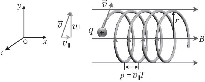
The pitch of the helix (distance advanced per revolution) is:
[EQUATION: Pitch = v_parallel × T = v_parallel × (2πm)/(qB)]
Common Error Alert: Many students assume magnetic fields can change a particle’s speed. Remember that magnetic forces are always perpendicular to velocity, so they can only change direction, never speed or kinetic energy.
Applications in Technology and Research
Mass Spectrometry:
Mass spectrometers use magnetic fields to separate ions based on their mass-to-charge ratios. Lighter ions follow tighter curves and arrive at detectors sooner than heavier ions with the same charge.
Particle Beam Focusing:
Magnetic lenses in electron microscopes focus particle beams by controlling their trajectories, enabling unprecedented resolution in imaging atomic structures.
Plasma Confinement:
In fusion reactors, powerful magnetic fields confine hot plasma by forcing charged particles to follow tight helical paths, preventing them from striking reactor walls.
Velocity Selectors and Crossed Fields
When electric and magnetic fields are perpendicular to each other and to a particle’s initial velocity, particles with specific velocities can travel undeflected:
[EQUATION: v = E/B for undeflected particles]
This principle enables velocity selectors that filter particles by speed, crucial for creating monoenergetic particle beams.
Problem-Solving Strategy: For complex trajectories, separate the motion into components parallel and perpendicular to the magnetic field. Analyze each component separately, then combine the results to understand the complete motion.
4: Force on Current-Carrying Conductors – Macroscopic Electromagnetic Effects
From Microscopic to Macroscopic Forces
While individual charges experience forces in magnetic fields, the practical applications of electromagnetism involve forces on current-carrying conductors. This transition from microscopic particle motion to macroscopic conductor forces bridges theoretical physics and engineering applications.
Consider a conductor carrying current I through a magnetic field B. Each charge carrier experiences a force, and the collective effect on all carriers creates a net force on the conductor:
[EQUATION: F = I(L × B) = ILB sin θ, where L is length vector along current direction]
This force per unit length relationship forms the basis for electric motors, generators, and electromagnetic actuators.
Direction Determination: Multiple Right-Hand Rules
Three equivalent methods exist for determining force direction on current-carrying conductors:
Method 1 – Current Direction:
- Point fingers along current direction
- Curl fingers toward magnetic field direction
- Thumb points in force direction
Method 2 – Charge Motion:
- Consider positive charge motion (current direction)
- Apply standard right-hand rule for moving charges
- Force direction applies to entire conductor
Method 3 – Vector Cross Product:
Use F = IL × B directly with vector mathematics
Physics Check: A horizontal wire carrying current from west to east lies in a vertical magnetic field pointing upward. What is the force direction on the wire? Using any right-hand rule method, the force points northward.
Forces Between Current-Carrying Conductors
Two parallel conductors carrying current exert forces on each other through their magnetic fields. This phenomenon, discovered by Ampère, provides the fundamental basis for defining the ampere as an SI base unit.
For two long parallel wires separated by distance d:
[EQUATION: F/L = (μ₀I₁I₂)/(2πd)]
Force Behavior:
- Parallel currents (same direction) → Attractive force
- Antiparallel currents (opposite directions) → Repulsive force
Real-World Physics: Power transmission lines carrying high currents must be carefully spaced to prevent mechanical damage from electromagnetic forces during fault conditions. Engineers design support structures to withstand these enormous forces.
Torque on Current Loops: The Foundation of Motors
When a current-carrying loop is placed in a magnetic field, it generally experiences a torque that tends to rotate it. This principle underlies all electric motors and moving-coil meters.
For a rectangular loop with current I in uniform field B:
[EQUATION: τ = NIAB sin θ, where N is number of turns, A is loop area, and θ is angle between field and loop normal]
Magnetic Dipole Moment:
The current loop behaves as a magnetic dipole with moment:
[EQUATION: μ = NIA, with direction given by right-hand rule]
The torque can then be expressed as:
[EQUATION: τ = μ × B]
Common Error Alert: The angle θ in torque calculations is measured from the field direction to the loop’s normal (perpendicular to the loop plane), not to the loop plane itself. Maximum torque occurs when the loop plane is parallel to the field (θ = 90°).
Practical Applications in Technology
Electric Motors:
Motors operate by creating continuous rotation through switching current directions in rotor coils as they rotate. Commutators or electronic switching ensures the torque always acts in the same rotational direction.
Moving Coil Galvanometers:
These sensitive current detectors use the proportional relationship between current and deflection angle. A spring provides restoring torque proportional to deflection angle, creating a linear current-deflection relationship.
Loudspeakers:
Speaker cones attach to current-carrying coils in radial magnetic fields. Alternating current creates oscillating forces, moving the cone to produce sound waves.
Electromagnetic Brakes:
Eddy current brakes use induced currents in rotating conductors. The resulting forces oppose motion, providing smooth, wear-free braking for trains and industrial machinery.
Force and Energy Considerations
Work-Energy Theorem Applications:
When magnetic forces move conductors, they can perform work and transfer energy. However, the magnetic field itself stores no energy – energy comes from the current source maintaining the current against induced EMF.
Power Considerations:
In motors, electrical power input converts to mechanical power output plus losses:
[EQUATION: P_electrical = P_mechanical + P_losses]
The efficiency depends on minimizing resistive heating and magnetic core losses.
Problem-Solving Strategy: When analyzing conductor forces, always consider:
- Current direction and magnitude
- Magnetic field direction and strength
- Conductor orientation relative to field
- Whether motion will occur and its direction
- Energy conservation implications
5: Magnetic Field Due to Current – Creating and Controlling Magnetic Fields
Biot-Savart Law Applications: Building Field Intuition
The Biot-Savart law provides the fundamental tool for calculating magnetic fields, but applying it effectively requires developing intuition about how current elements contribute to total fields.
Straight Wire Field Analysis:
For a finite straight wire, the field calculation involves integrating contributions from each current element:
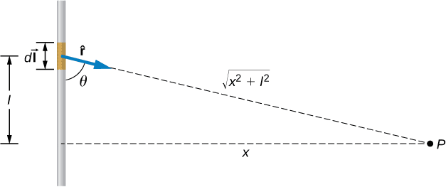
The resulting field at perpendicular distance r from a wire of length L:
[EQUATION: B = (μ₀I/4πr)[sin θ₂ – sin θ₁], where θ₁ and θ₂ are angles from wire ends to field point]
For an infinite wire, this simplifies to the familiar result:
[EQUATION: B = μ₀I/(2πr)]
Physics Check: How does the field 2 meters from a long straight wire compare to the field 1 meter away? Since field is inversely proportional to distance, the field at 2 meters is exactly half the field at 1 meter.
Circular Current Loops: Symmetry and Field Patterns
Circular current loops create magnetic fields with beautiful symmetry properties. At the center of a single-turn loop:
[EQUATION: B = μ₀I/(2R)]
For N turns in a tightly wound coil:
[EQUATION: B = μ₀NI/(2R)]
Field Along the Axis:
The field along the axis of a circular loop provides insight into how field strength varies with position:
[EQUATION: B = (μ₀IR²)/(2(R² + x²)³/²), where x is distance along axis from loop center]
This equation shows how the field decreases as you move away from the loop along its axis.
Real-World Physics: Helmholtz coils consist of two identical circular coils separated by a distance equal to their radius. This configuration creates an extremely uniform magnetic field in the region between the coils, essential for calibrating magnetic instruments and shielding sensitive experiments.
Solenoids: Uniform Fields and Practical Applications
A solenoid is a tightly wound coil of wire, typically cylindrical, that creates a uniform magnetic field inside while producing minimal field outside. This makes solenoids ideal for creating controlled magnetic environments.
Inside a Long Solenoid:
[EQUATION: B = μ₀nI, where n = N/L is turns per unit length]
Outside a Long Solenoid:
B ≈ 0 (negligible field outside an ideal solenoid)
Field Direction:
Use the right-hand rule: curl fingers in current direction, thumb points toward the north pole of the solenoid.
Common Error Alert: The uniform field formula B = μ₀nI applies only inside long solenoids where end effects are negligible. Near the ends, the field strength is approximately half the interior value.
Ampère’s Circuital Law: Exploiting Symmetry
Ampère’s law provides an elegant method for calculating fields when current distributions have appropriate symmetry:
[EQUATION: ∮ B⃗ · dl⃗ = μ₀I_enclosed]
Choosing Amperian Loops:
The key to using Ampère’s law effectively is choosing loops that match the symmetry of the problem:
- Circular loops for cylindrical symmetry (straight wires, cylindrical conductors)
- Rectangular loops for planar symmetry (infinite current sheets)
- Loops that exploit field symmetries and zeros
Inside a Current-Carrying Cylinder:
For a solid cylindrical conductor of radius R carrying current I uniformly distributed:
- Inside (r < R): B = (μ₀Ir)/(2πR²)
- Outside (r > R): B = μ₀I/(2πr)
Current Sheets:
An infinite sheet of current with surface current density K creates:
[EQUATION: B = μ₀K/2, independent of distance from sheet]
Toroidal Coils: Confining Magnetic Fields
Toroidal (doughnut-shaped) coils demonstrate how geometry can completely confine magnetic fields:
Inside the Torus:
[EQUATION: B = μ₀NI/(2πr), where r is distance from torus center]
Outside the Torus:
B = 0 (all magnetic field lines are contained within the torus)
This complete field confinement makes toroids ideal for transformers and inductors where field leakage must be minimized.
Historical Context: The discovery that magnetic fields could be completely contained within certain geometries revolutionized electrical engineering, leading to more efficient transformers and reduced electromagnetic interference in electronic devices.
Superposition and Field Addition
When multiple current sources exist, the total magnetic field equals the vector sum of individual contributions:
[EQUATION: B⃗_total = B⃗₁ + B⃗₂ + B⃗₃ + …]
Vector Addition Strategies:
- Calculate each field contribution separately
- Determine field directions using right-hand rules
- Add components algebraically (use coordinate systems)
- Find resultant magnitude and direction
Problem-Solving Strategy: For complex current configurations:
- Identify symmetries that simplify calculations
- Break complex shapes into standard geometries
- Use superposition to combine field contributions
- Check limiting cases (very close, very far, along symmetry axes)
Real-World Physics: MRI machines use multiple coils with precisely calculated current patterns to create uniform fields over large volumes. Computer simulations optimize coil positions and currents to achieve the required field uniformity for medical imaging.
6: Advanced Applications and Modern Technology
Electromagnetic Induction Preview: Dynamic Fields
While electromagnetic induction is covered in detail in the next chapter, understanding how changing magnetic fields create electric fields provides crucial context for many applications of moving charges and magnetism.
Faraday’s Law Connection:
When conductors move through magnetic fields or when magnetic fields change with time, electric fields are induced. This reciprocal relationship between electricity and magnetism underlies:
- Electric generators converting mechanical energy to electrical energy
- Transformers changing voltage levels in power distribution
- Induction motors and wireless charging systems
Lenz’s Law and Energy Conservation:
The direction of induced effects always opposes the change causing them, ensuring energy conservation in electromagnetic systems.
Particle Accelerators: Ultimate Applications
Modern particle accelerators represent the most sophisticated applications of electromagnetic principles, pushing charged particles to velocities approaching the speed of light.
Cyclotrons:
Traditional cyclotrons use the constant cyclotron frequency in uniform magnetic fields:
- Particles spiral outward as they gain energy
- Radio frequency acceleration synchronizes with particle motion
- Maximum energy limited by relativistic effects
Synchrotrons:
Advanced accelerators vary magnetic field strength to maintain constant orbital radius:
- Particles maintain fixed orbital paths while gaining energy
- Superconducting magnets create extremely strong, stable fields
- Applications include high-energy physics research and medical treatments
Linear Accelerators (LINACs):
Use alternating electric fields for acceleration with magnetic fields for beam focusing:
- No energy limit from curved paths
- Require precise beam control using magnetic focusing elements
- Used in cancer treatment and materials research
Magnetic Resonance Imaging: Physics Serving Medicine
MRI technology demonstrates the practical application of magnetic field theory to medical diagnosis:
Field Requirements:
- Uniform main field (typically 1.5-3 Tesla) for consistent signal
- Gradient coils create controlled field variations for spatial encoding
- RF coils generate and detect electromagnetic signals
Physics Principles:
- Hydrogen nuclei in body tissues act as tiny magnetic dipoles
- Strong magnetic fields align these dipoles
- Radio frequency pulses tip dipoles out of alignment
- Relaxation back to equilibrium creates detectable signals
Safety Considerations:
The powerful magnetic fields in MRI machines create significant safety challenges:
- Ferromagnetic objects become dangerous projectiles
- Induced currents in conductive implants can cause heating
- Gradient field switching creates acoustic noise
Magnetic Levitation: Frictionless Transportation
Magnetic levitation (maglev) technology uses electromagnetic forces to suspend and propel vehicles without physical contact:
Electromagnetic Suspension (EMS):
- Electromagnets attract to ferromagnetic rails
- Active control systems maintain stable gaps
- Used in some commercial maglev trains
Electrodynamic Suspension (EDS):
- Superconducting magnets interact with induced currents in track conductors
- Naturally stable levitation above threshold speed
- Higher operating speeds than EMS systems
Linear Motors:
- Track acts as motor stator, vehicle carries moving magnetic field
- Precise control of propulsion forces
- Regenerative braking recovers energy during deceleration
Plasma Physics and Fusion Research
Controlled fusion research relies heavily on magnetic confinement of high-temperature plasmas:
Tokamaks:
- Twisted magnetic field lines confine plasma particles
- Combination of toroidal and poloidal field components
- Superconducting coils create stable, long-duration confinement
Magnetic Bottle Configuration:
- Converging magnetic field lines create particle traps
- Used in smaller-scale plasma experiments
- Demonstrates basic principles of magnetic confinement
Particle Transport:
- Charged particles follow magnetic field lines
- Collisions cause gradual drift across field lines
- Understanding transport physics crucial for fusion reactor design
Electromagnetic Compatibility and Shielding
Modern electronics must coexist without mutual interference:
Shielding Principles:
- Conducting enclosures redirect magnetic fields around sensitive components
- High-permeability materials concentrate fields away from protected areas
- Proper grounding prevents unwanted current loops
EMI/EMC Standards:
- Regulations limit electromagnetic emissions from devices
- Susceptibility testing ensures proper operation in electromagnetic environments
- Design considerations include cable routing and circuit layout
Common Error Alert: Many students think any conducting material provides complete electromagnetic shielding. In reality, shielding effectiveness depends on material properties, thickness, frequency, and construction details like seam integrity.
7: Laboratory Investigations and Experimental Skills
Measuring Magnetic Fields: Instruments and Techniques
Understanding how to measure and characterize magnetic fields is essential for both academic study and practical applications.
Hall Effect Probes:
- Semiconductor devices that generate voltage proportional to magnetic field
- Can measure both field magnitude and direction
- Useful for mapping field distributions around current-carrying conductors
Search Coils:
- Coils of wire that generate voltage when moved through magnetic fields
- Voltage proportional to rate of flux change
- Useful for measuring field gradients and studying field patterns
Fluxgate Magnetometers:
- Highly sensitive instruments using magnetic core saturation
- Can detect very weak fields (nanotesla range)
- Used in geophysical surveys and space research
Demonstrating Fundamental Principles
Oersted’s Experiment (Current Creates Magnetic Field):
Setup: Compass needle near current-carrying wire
Observation: Needle deflection proportional to current
Analysis: Demonstrates magnetic field circulation around current
Force on Current-Carrying Conductor:
Setup: Flexible conductor in magnetic field between permanent magnets
Observation: Conductor deflection when current flows
Analysis: Quantifies relationship between current, field, and force
Charged Particle Deflection:
Setup: Electron beam (cathode ray tube) with external magnetic field
Observation: Curved electron path in presence of magnetic field
Analysis: Determines electron charge-to-mass ratio
Error Analysis and Uncertainty Estimation
Systematic Errors:
- Instrument calibration errors affect all measurements consistently
- Magnetic field inhomogeneities create position-dependent errors
- Temperature effects on permanent magnets and electronic instruments
Random Errors:
- Electrical noise in sensitive measurements
- Mechanical vibrations affecting delicate apparatus
- Human reaction time in manual timing measurements
Uncertainty Propagation:
When calculating derived quantities, uncertainties combine according to:
- Addition/subtraction: Add absolute uncertainties
- Multiplication/division: Add relative uncertainties
- Powers: Multiply relative uncertainty by power
Measurement Techniques:
- Multiple measurements reduce random errors
- Calibration against known standards eliminates systematic errors
- Proper instrument selection matches precision to measurement requirements
Safety Considerations in Electromagnetic Experiments
High Current Safety:
- Proper fusing and circuit breakers prevent dangerous overcurrents
- Heat dissipation considerations for high-power experiments
- Awareness of magnetic forces on ferromagnetic tools and implants
Strong Magnetic Fields:
- Keep magnetic storage media away from strong fields
- Understand effects on electronic devices (phones, computers, pacemakers)
- Proper handling and storage of permanent magnets
Electrical Safety:
- Proper grounding of all apparatus
- Understanding of electrical shock hazards
- Emergency procedures for electrical accidents
Real-World Physics: Professional research laboratories use sophisticated safety protocols when working with superconducting magnets that can generate fields over 20 Tesla – strong enough to levitate a frog through diamagnetic effects!
Practice Problems Section: Mastering Moving Charges and Magnetism
Level 1: Fundamental Concepts (Basic Understanding)
Problem 1: A proton (charge = +1.6 × 10⁻¹⁹ C, mass = 1.67 × 10⁻²⁷ kg) enters a uniform magnetic field of 0.5 T with velocity 2 × 10⁶ m/s perpendicular to the field. Calculate the radius of its circular path.
Solution:
Using the formula for radius of circular motion in magnetic field:
r = mv/(qB)
r = (1.67 × 10⁻²⁷ kg)(2 × 10⁶ m/s)/[(1.6 × 10⁻¹⁹ C)(0.5 T)]
r = (3.34 × 10⁻²¹)/(8 × 10⁻²⁰) = 0.042 m = 4.2 cm
Problem 2: A straight wire carries a current of 5 A. Calculate the magnetic field at a distance of 10 cm from the wire.
Solution:
Using Biot-Savart law for infinite straight wire:
B = μ₀I/(2πr)
B = (4π × 10⁻⁷ T·m/A)(5 A)/[2π(0.1 m)]
B = (20π × 10⁻⁷)/(0.2π) = 1 × 10⁻⁵ T = 10 μT
Problem 3: A rectangular loop with dimensions 20 cm × 30 cm carries a current of 2 A. The loop is placed in a uniform magnetic field of 0.8 T with its plane making an angle of 60° with the field direction. Calculate the torque on the loop.
Solution:
Torque τ = NIAB sin θ, where θ is angle between field and loop normal
Since plane makes 60° with field, normal makes 30° with field
τ = (1)(2 A)(0.2 m × 0.3 m)(0.8 T) sin 30°
τ = (2)(0.06)(0.8)(0.5) = 0.048 N·m
Level 2: Intermediate Applications (Problem-Solving Skills)
Problem 4: An electron moving with velocity 5 × 10⁷ m/s enters a region where both electric field (200 N/C) and magnetic field (0.01 T) exist perpendicular to each other and to the electron’s velocity. Find the condition for the electron to move undeflected.
Solution:
For undeflected motion, electric and magnetic forces must balance:
qE = qvB (magnitudes, forces in opposite directions for negative charge)
E = vB
v = E/B = (200 N/C)/(0.01 T) = 2 × 10⁴ m/s
Since given velocity (5 × 10⁷ m/s) ≠ required velocity (2 × 10⁴ m/s), the electron will be deflected.
Problem 5: Two parallel wires separated by 5 cm carry currents of 3 A and 4 A in the same direction. Calculate the force per unit length between them.
Solution:
Force per unit length between parallel current-carrying conductors:
F/L = (μ₀I₁I₂)/(2πd)
F/L = (4π × 10⁻⁷ T·m/A)(3 A)(4 A)/[2π(0.05 m)]
F/L = (48π × 10⁻⁷)/(0.1π) = 4.8 × 10⁻⁵ N/m
Since currents are in same direction, force is attractive.
Problem 6: A solenoid with 2000 turns and length 50 cm carries a current of 1.5 A. Calculate the magnetic field inside the solenoid.
Solution:
For a long solenoid: B = μ₀nI, where n = N/L
n = 2000 turns/0.5 m = 4000 turns/m
B = (4π × 10⁻⁷ T·m/A)(4000 turns/m)(1.5 A)
B = (4π × 10⁻⁷)(6000) = 7.54 × 10⁻³ T = 7.54 mT
Level 3: Advanced Problem Solving (Synthesis and Analysis)
Problem 7: A charged particle with q/m = 2 × 10⁸ C/kg enters a magnetic field region with velocity components vₓ = 3 × 10⁶ m/s and vᵧ = 4 × 10⁶ m/s. The magnetic field B = 0.1 T points in the z-direction. Describe the particle’s motion and calculate relevant parameters.
Solution:
Initial speed: v = √(vₓ² + vᵧ²) = √(9 + 16) × 10⁶ = 5 × 10⁶ m/s
The particle will follow a circular path in the x-y plane with:
Cyclotron frequency: ω = qB/m = (2 × 10⁸)(0.1) = 2 × 10⁷ rad/s
Period: T = 2π/ω = π × 10⁻⁷ s
Radius: r = mv/(qB) = v/(qB/m) = (5 × 10⁶)/(2 × 10⁷) = 0.25 m
Problem 8: A circular coil of 100 turns with radius 5 cm is placed coaxially with a long solenoid. The solenoid has 2000 turns over 40 cm length. If the current in the solenoid is increasing at 50 A/s, find the induced EMF in the coil.
Solution:
First, find the magnetic field inside the solenoid:
B = μ₀nI = μ₀(2000/0.4)I = μ₀(5000)I
The flux through the coil (assuming coil is entirely within solenoid):
Φ = BA = μ₀(5000)I × π(0.05)² = μ₀(5000)I × π(2.5 × 10⁻³)
Induced EMF: ε = -N(dΦ/dt) = -100 × μ₀(5000) × π(2.5 × 10⁻³) × (dI/dt)
ε = -100 × (4π × 10⁻⁷) × 5000 × π × 2.5 × 10⁻³ × 50
ε = -100 × 4π² × 10⁻⁷ × 5000 × 2.5 × 10⁻³ × 50
ε = -2.47 × 10⁻³ V = -2.47 mV
Level 4: CBSE Board Exam Style Questions
Problem 9: [Multiple Choice] A charged particle moving in a magnetic field follows a helical path. This happens when:
(a) Velocity is parallel to magnetic field
(b) Velocity is perpendicular to magnetic field
(c) Velocity has components both parallel and perpendicular to magnetic field
(d) Magnetic field varies with position
Answer: (c) – Helical motion results from superposition of circular motion (perpendicular component) and linear motion (parallel component).
Problem 10: [Numerical] A uniform magnetic field of 1.5 T exists in a cylindrical region of radius 10 cm. An electron enters this region with velocity 2 × 10⁷ m/s perpendicular to the field at the edge of the region. Will the electron complete a full circle inside the magnetic field region? Justify your answer with calculations.
Solution:
Radius of electron’s circular path:
r = mv/(eB) = (9.1 × 10⁻³¹ kg)(2 × 10⁷ m/s)/[(1.6 × 10⁻¹⁹ C)(1.5 T)]
r = (18.2 × 10⁻²⁴)/(2.4 × 10⁻¹⁹) = 0.076 m = 7.6 cm
Since the radius of the electron’s path (7.6 cm) is less than the radius of the magnetic field region (10 cm), the electron will complete a full circle inside the field region.
Problem 11: [Theory + Numerical] Derive an expression for the magnetic field at the center of a circular current loop. Use this to find the field when 20 turns of wire carrying 2 A current form a coil of radius 8 cm.
Solution:
Derivation: Using Biot-Savart law for a circular loop
Each element contributes: dB = (μ₀I dl)/(4πr²)
Since dl and r are perpendicular for all elements, and r is constant:
B = ∫dB = (μ₀I)/(4πR²) ∫dl = (μ₀I)/(4πR²) × 2πR = μ₀I/(2R)
Numerical Calculation:
For N turns: B = μ₀NI/(2R)
B = (4π × 10⁻⁷ T·m/A)(20)(2 A)/[2(0.08 m)]
B = (4π × 10⁻⁷)(40)/(0.16) = π × 10⁻⁴ T = 3.14 × 10⁻⁴ T
Level 5: Conceptual and Analytical Questions
Problem 12: Explain why magnetic forces cannot change the kinetic energy of a charged particle. How does this principle apply to particle accelerators?
Answer:
Magnetic forces are always perpendicular to particle velocity (F = q v × B). Since work is defined as W = F · ds = F · v dt, and the magnetic force is perpendicular to velocity, no work is done by magnetic forces. Therefore, kinetic energy remains constant.
In particle accelerators:
- Magnetic fields are used for steering and focusing, not acceleration
- Electric fields provide acceleration (increase kinetic energy)
- Magnetic fields control particle trajectories without energy change
- This allows precise beam control while maintaining particle energies
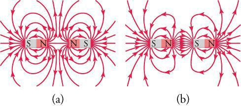
Problem 13: Compare and contrast the magnetic field patterns inside and outside a solenoid with those of a bar magnet. Explain the similarities and differences.
Answer:
Similarities:
- Both create dipole field patterns with distinct north and south poles
- Field lines are continuous loops from north to south pole
- Field strength decreases with distance outside the source
Differences:
- Solenoid: Uniform field inside, negligible field outside (ideal case)
- Bar magnet: Non-uniform field everywhere, significant external field
- Solenoid: Field strength controllable via current
- Bar magnet: Fixed field strength (permanent magnetization)
- Solenoid: Field direction reversible by changing current direction
- Bar magnet: Fixed polarity (unless remagnetized)
Physical Origin:
- Solenoid: Organized current loops create controlled field pattern
- Bar magnet: Aligned atomic magnetic dipoles create net field
Problem 14: A student claims that increasing the number of turns in a solenoid will always increase the magnetic field inside. Under what conditions might this claim be incorrect?
Answer:
The claim may be incorrect under several conditions:
Current Limitation:
If total resistance increases significantly with more turns, and voltage source is fixed, current may decrease enough to offset the benefit of additional turns.
Self-Inductance Effects:
More turns increase self-inductance, which can limit current rise time in AC applications.
Geometric Constraints:
If solenoid length increases proportionally with turns, the field remains B = μ₀nI (unchanged).
Saturation Effects:
With ferromagnetic cores, additional turns may not increase field if core material saturates.
Correct Statement:
Increasing turn density (turns per unit length) while maintaining constant current always increases field strength inside a solenoid.
Exam Preparation Strategies: Mastering Board Exam Success
Understanding CBSE Physics Paper Pattern
Section Allocation for Moving Charges and Magnetism:
- Multiple Choice Questions (1 mark each): 2-3 questions typically focus on conceptual understanding and formula applications
- Short Answer Questions (2 marks each): 1-2 questions requiring brief explanations or simple calculations
- Long Answer Questions (3-5 marks each): 1 major question involving detailed problem-solving or derivations
- Total weightage: Approximately 8-12 marks out of 70 total marks
Common Question Types:
- Derivation Questions: Magnetic field due to straight wire, circular loop, or solenoid
- Force Calculations: Lorentz force on charged particles, forces between conductors
- Circular Motion Problems: Radius, frequency, and energy relationships
- Conceptual Questions: Right-hand rules, field line properties, energy considerations
- Application Problems: Real-world scenarios involving electromagnetic devices
Formula Sheet and Key Relationships
Essential Formulas for Quick Reference:
Lorentz Force:
- F = q(v × B) = qvB sin θ
- For circular motion: r = mv/(qB), f = qB/(2πm)
Magnetic Fields Due to Currents:
- Straight wire: B = μ₀I/(2πr)
- Circular loop center: B = μ₀I/(2R)
- Solenoid interior: B = μ₀nI
Forces on Conductors:
- Single conductor: F = IL × B = ILB sin θ
- Between parallel wires: F/L = μ₀I₁I₂/(2πd)
- Torque on loop: τ = NIAB sin θ
Fundamental Constants:
- μ₀ = 4π × 10⁻⁷ T·m/A
- e = 1.6 × 10⁻¹⁹ C
- mₑ = 9.1 × 10⁻³¹ kg
- mₚ = 1.67 × 10⁻²⁷ kg
Conclusion: Connecting Electromagnetic Theory to Future Learning
Integration with Other Physics Units
The principles you’ve mastered in Moving Charges and Magnetism serve as crucial foundations for understanding advanced physics concepts throughout your CBSE Class 12 curriculum and beyond.
Electromagnetic Induction (Next Chapter):
Your understanding of magnetic fields and their interactions with moving charges directly enables comprehension of how changing magnetic fields induce electric fields. The reciprocal relationship between electricity and magnetism becomes complete when you study Faraday’s law and Lenz’s law.
Alternating Current Physics:
The concepts of magnetic flux and field interactions with conductors provide the theoretical foundation for understanding transformers, inductors, and AC motor operation. Your knowledge of force relationships explains how AC motors convert electrical energy to mechanical work.
Modern Physics Applications:
The charged particle motion principles you’ve learned are fundamental to understanding:
- Atomic structure and electron orbital behavior
- Mass spectrometry and particle detection techniques
- Quantum mechanical magnetic moments and spin interactions
- Relativistic effects in high-energy particle physics
Real-World Career Connections
Electrical and Electronics Engineering:
Every motor, generator, transformer, and electromagnetic device relies on the principles you’ve studied. Understanding magnetic field calculations and force relationships enables design of efficient electrical machines and power systems.
Medical Physics and Bioengineering:
MRI technology, electromagnetic therapy devices, and biomedical instrumentation all apply electromagnetic principles. Your foundation in field theory and particle motion prepares you for advanced medical technology careers.
Research and Development:
Particle accelerator design, fusion energy research, and electromagnetic compatibility testing all require deep understanding of charged particle motion and magnetic field control.
Space Technology:
Satellite attitude control, plasma propulsion systems, and radiation shielding all utilize electromagnetic principles. Your understanding of particle trajectories in magnetic fields is essential for space technology development.
Preparation for Advanced Studies
University Physics:
The vector analysis skills, field theory concepts, and problem-solving approaches you’ve developed provide essential preparation for advanced electromagnetic theory, including Maxwell’s equations and wave propagation.
Engineering Applications:
Whether you pursue electrical, mechanical, aerospace, or biomedical engineering, the electromagnetic principles from this chapter appear repeatedly in advanced coursework and professional practice.
Research Opportunities:
Understanding electromagnetic phenomena opens doors to research in areas ranging from renewable energy technology to quantum computing and space exploration.
Final Thoughts: The Beauty of Electromagnetic Unity
As you complete your study of Moving Charges and Magnetism, reflect on the elegant unity of electromagnetic phenomena. The same principles that govern a simple compass needle also control the massive electromagnets in particle accelerators and the delicate magnetic fields in your smartphone’s speakers.
This chapter represents a crucial step in your physics education, connecting the static world of electrostatics to the dynamic realm of electromagnetic fields. You’ve gained tools that will serve you throughout your scientific and technical career, whether you become an engineer designing the next generation of electric vehicles, a researcher probing the mysteries of plasma physics, or simply an educated citizen who understands the electromagnetic foundations of modern technology.
The mathematics you’ve mastered, the physical intuition you’ve developed, and the problem-solving strategies you’ve practiced all contribute to a deeper appreciation of the natural world and our technological achievements. As you progress to study electromagnetic induction, alternating current phenomena, and eventually Maxwell’s complete theory of electromagnetism, remember that every advance builds upon the solid foundation you’ve established through mastering moving charges and magnetism.
Your journey through physics continues to reveal the profound connections between mathematical beauty and physical reality. The invisible forces you’ve learned to calculate and predict shape the visible world around us in ways both subtle and dramatic. This knowledge empowers you to understand, create, and innovate in our increasingly electromagnetic world.
Continue to approach physics with curiosity, persistence, and appreciation for the elegant simplicity underlying apparent complexity. The electromagnetic principles you’ve mastered represent humanity’s hard-won understanding of some of nature’s most fundamental forces – knowledge that continues to drive technological progress and expand our understanding of the universe itself.
This comprehensive study guide provides the foundation for excellence in CBSE Class 12 Physics Unit 3: Chapter 4 – Moving Charges and Magnetism. Continue practicing regularly, maintain curiosity about electromagnetic phenomena in daily life, and approach your board exam with confidence in your thorough preparation.
Recommended –
2 thoughts on “CBSE Class 12 Physics: Chapter 4 – Moving Charges and Magnetism: Complete Study Guide for Exam Success”