

Have you ever wondered why a guitar string produces the exact same pitch every time you pluck it? Or how your smartphone’s screen responds so precisely to your touch? The answer lies in one of physics’ most elegant and ubiquitous phenomena: oscillations. From the pendulum in your grandfather’s clock to the atoms vibrating in your coffee mug, oscillatory motion governs countless aspects of our world.
As an AP Physics 1 student, Unit 7: Oscillations represents a fascinating convergence of everything you’ve learned so far-forces, energy, momentum, and waves all come together in the rhythmic dance of periodic motion. This comprehensive guide will transform you from someone who simply recognizes oscillations to someone who truly understands the profound physics principles that make your world tick, vibrate, and resonate.
What You’ll Master in Unit 7
By the end of this unit, you’ll have developed a deep understanding of oscillatory systems that will serve you well beyond the AP exam. Specifically, you’ll be able to:
- Analyze simple harmonic motion using both energy and force approaches
- Derive and apply the mathematical relationships governing pendulums and mass-spring systems
- Predict and explain how changing physical parameters affects oscillatory behavior
- Design experiments to investigate oscillatory motion and analyze the resulting data
- Connect oscillations to wave phenomena and real-world applications
- Solve complex problems involving multiple oscillating systems
These objectives align directly with the College Board’s Essential Knowledge statements 7.A.1 through 7.A.4, ensuring you’re fully prepared for both the multiple-choice and free-response sections of the AP exam.
The Foundation: Understanding Periodic Motion
Picture yourself on a swing at your local playground. As you pump your legs and soar through the air, you’re experiencing one of nature’s most fundamental patterns: periodic motion. Every oscillating system, from atomic vibrations to planetary orbits, shares certain key characteristics that make them predictable and mathematically elegant.
Periodic motion occurs when an object repeats the same motion over and over again in fixed intervals of time. The time required for one complete cycle is called the period (T), measured in seconds. The number of complete cycles that occur in one second is the frequency (f), measured in hertz (Hz). These quantities are inversely related: f = 1/T.
But here’s where it gets interesting from a physics perspective. Not all periodic motion is created equal. The special case we call simple harmonic motion (SHM) occurs when the restoring force acting on an object is directly proportional to its displacement from equilibrium and acts in the opposite direction. Mathematically, this relationship appears as:
F = -kx
where k is a positive constant and x represents displacement from the equilibrium position.
Real-World Physics: The negative sign in this equation isn’t just mathematical formality-it represents something profound about nature. Systems naturally tend toward equilibrium, and the farther you push them away, the harder they push back. This principle governs everything from the springs in your car’s suspension to the molecular bonds that hold your DNA together.
Simple Harmonic Motion: The Mathematics of Natural Rhythm
When we say an object undergoes simple harmonic motion, we’re making a specific claim about the nature of the forces acting on it. Let’s dive deep into what this means and why it matters for your AP Physics success.
The Position Equation
For an object in simple harmonic motion, the position as a function of time follows a sinusoidal pattern:
x(t) = A cos(ωt + φ)
where:
- A is the amplitude (maximum displacement from equilibrium)
- ω is the angular frequency (ω = 2πf = 2π/T)
- φ is the phase constant (determines the initial conditions)
- t is time
This equation might look intimidating at first, but think of it as a mathematical description of smooth, rhythmic motion. The cosine function naturally oscillates between +1 and -1, so when multiplied by the amplitude A, it gives us the actual position oscillating between +A and -A.
Velocity and Acceleration in SHM
Taking the derivative of position gives us velocity:
v(t) = -Aω sin(ωt + φ)
Notice that velocity reaches its maximum value of Aω when the object passes through equilibrium (x = 0), and velocity equals zero at the turning points where x = ±A.
Taking another derivative gives us acceleration:
a(t) = -Aω² cos(ωt + φ) = -ω²x(t)
This final relationship, a = -ω²x, is perhaps the most important equation in all of oscillatory motion. It tells us that acceleration is always proportional to displacement but in the opposite direction-exactly what we’d expect from our force equation F = -kx combined with Newton’s second law.
Physics Check: Can you see why the acceleration is maximum when the object is at its maximum displacement? This makes intuitive sense-when a spring is stretched the farthest, it exerts the strongest restoring force, producing the greatest acceleration back toward equilibrium.
Energy in Simple Harmonic Motion
One of the most beautiful aspects of simple harmonic motion is how energy continuously transforms between kinetic and potential forms while the total mechanical energy remains constant (assuming no friction).
For a mass-spring system:
- Kinetic Energy: KE = ½mv² = ½mA²ω² sin²(ωt + φ)
- Potential Energy: PE = ½kx² = ½kA² cos²(ωt + φ)
- Total Energy: E = KE + PE = ½kA² = ½mA²ω²
The total energy is proportional to the square of the amplitude-double the amplitude, and you quadruple the energy. This relationship has profound implications for everything from earthquake damage (larger amplitude seismic waves carry exponentially more destructive energy) to the design of musical instruments.
Common Physics Mistake Alert: Students often assume that maximum kinetic energy occurs at maximum displacement. In reality, kinetic energy is maximum at equilibrium (where velocity is maximum) and zero at the turning points (where velocity is zero). This is opposite to potential energy, which is maximum at the turning points and zero at equilibrium.
The Mass-Spring System: Engineering Oscillations
The mass-spring system represents the archetypal example of simple harmonic motion, and understanding it thoroughly will serve as your foundation for analyzing more complex oscillatory systems.
Deriving the Period Formula
When a mass m is attached to a spring with spring constant k, the restoring force follows Hooke’s law: F = -kx. Applying Newton’s second law:
ma = -kx
m(d²x/dt²) = -kx
d²x/dt² = -(k/m)x
Comparing this to our standard SHM equation a = -ω²x, we can identify:
ω² = k/m
Therefore: ω = √(k/m)
And since T = 2π/ω:
T = 2π√(m/k)
This elegant formula tells us something remarkable: the period of a mass-spring system depends only on the mass and the spring constant, not on the amplitude of oscillation. You can stretch the spring a little or a lot-as long as you stay within the elastic limit, the period remains the same.
Problem-Solving Strategy: When analyzing mass-spring systems, always start by identifying the equilibrium position. This is where the gravitational force exactly balances the spring force, and it serves as your reference point for measuring displacement in the SHM equations.
Vertical Mass-Spring Systems
When dealing with a mass hanging from a vertical spring, many students get confused about how gravity affects the motion. Here’s the key insight: gravity simply shifts the equilibrium position downward by an amount equal to mg/k, but it doesn’t change the period or frequency of oscillation.
At the new equilibrium position:
kx₀ = mg
x₀ = mg/k
If you measure all displacements from this new equilibrium position, the motion follows standard SHM with the same period T = 2π√(m/k).
Real-World Physics: This principle explains why your car’s suspension system works effectively regardless of whether you’re driving uphill, downhill, or on level ground. The springs automatically adjust to a new equilibrium position based on the car’s orientation, but the oscillatory characteristics that provide a smooth ride remain unchanged.

Energy Analysis of Mass-Spring Systems
Let’s work through a comprehensive energy analysis that demonstrates the power of conservation principles in oscillatory motion.
Consider a 0.5 kg mass attached to a spring with k = 200 N/m, oscillating with an amplitude of 0.1 m. We can calculate:
Total Energy: E = ½kA² = ½(200)(0.1)² = 1.0 J
At maximum displacement (x = ±0.1 m):
- PE = ½kx² = ½(200)(0.1)² = 1.0 J
- KE = 0 J (velocity is zero at turning points)
At equilibrium (x = 0):
- PE = 0 J
- KE = 1.0 J = ½mv²max, so vmax = 2.0 m/s
At intermediate position (x = 0.05 m):
- PE = ½k(0.05)² = 0.25 J
- KE = E – PE = 1.0 – 0.25 = 0.75 J
This analysis demonstrates the continuous energy transformation that characterizes all oscillatory motion.
The Simple Pendulum: Gravity’s Timekeeper
The simple pendulum-a point mass suspended by a massless, inextensible string-has captivated physicists and engineers for centuries. From Galileo’s observations of swinging chandeliers to modern atomic clocks, pendulums have played a crucial role in our understanding of time and motion.
The Small Angle Approximation
For a pendulum of length L, the restoring torque about the pivot point is:
τ = -mgL sin θ
where θ is the angular displacement from vertical. For simple harmonic motion to occur, we need the restoring force to be proportional to displacement. This happens when we make the small angle approximation: for small angles (θ < 15°), sin θ ≈ θ (in radians).
With this approximation:
τ = -mgLθ
The rotational analog of Newton’s second law gives us:
Iα = -mgLθ
For a point mass at distance L: I = mL²
mL²α = -mgLθ
α = -(g/L)θ
Since α = d²θ/dt², this becomes:
d²θ/dt² = -(g/L)θ
Comparing to the standard SHM equation, we identify ω² = g/L, giving us:
T = 2π√(L/g)
This famous result tells us that the period of a simple pendulum depends only on its length and the acceleration due to gravity-not on the mass of the bob or the amplitude of oscillation (for small angles).
Physics Check: Why doesn’t the mass affect the period? It’s because both the restoring torque and the moment of inertia are proportional to mass, so the mass cancels out in the equation of motion. This is analogous to how mass cancels out in free fall problems.
Experimental Design: Measuring g with a Pendulum
The pendulum’s period formula provides an excellent opportunity to design an experiment for measuring local gravitational acceleration. Here’s a comprehensive experimental approach:
Hypothesis: The period of a simple pendulum is given by T = 2π√(L/g), so measuring T and L allows us to calculate g.
Variables:
- Independent: Length L (varied from 0.3 m to 1.5 m)
- Dependent: Period T (measured for each length)
- Controlled: Mass of bob, amplitude (kept small), string type
Procedure:
- Set up pendulum with measured length L
- Displace bob by small angle (< 10°)
- Release and time 20 complete oscillations
- Calculate period: T = (total time)/20
- Repeat for different lengths
- Plot T² vs. L (should be linear)
- Calculate g from slope: slope = 4π²/g
Data Analysis:
The theoretical relationship T² = (4π²/g)L suggests that a graph of T² versus L should yield a straight line with slope 4π²/g. Any deviation from linearity might indicate:
- Large angle effects
- Air resistance
- String stretching
- Timing errors
Error Analysis:
Major sources of uncertainty include:
- Measurement of length (±0.001 m)
- Timing precision (±0.01 s)
- Definition of “complete oscillation”
- Environmental factors (air currents, temperature)
This experiment beautifully demonstrates how simple harmonic motion connects to fundamental physical constants.


Physical Pendulum: Beyond the Simple Case
While the simple pendulum provides an elegant introduction to oscillatory motion, most real-world pendulums don’t behave as point masses. The physical pendulum-any rigid body that oscillates about a fixed axis-requires us to consider the distribution of mass throughout the object.
The Physical Pendulum Formula
For a physical pendulum with moment of inertia I about the pivot point, mass M, and distance d from the pivot to the center of mass:
T = 2π√(I/Mgd)
This reduces to the simple pendulum formula when I = ML² and d = L (for a point mass at distance L).
Real-World Physics: Consider a baseball bat swinging about your hands. The period depends not just on the bat’s length, but on how the mass is distributed along its length. A bat with more mass concentrated at the handle will oscillate differently than one with mass concentrated at the barrel, even if both have the same total mass and length.
Applications in Engineering
Physical pendulums find applications in numerous engineering contexts:
Seismographs: Earthquake detection relies on the predictable oscillation of suspended masses. When the ground moves, the pendulum’s inertia causes it to lag behind, creating relative motion that can be recorded.
Metronomes: The adjustable weight on a metronome effectively changes the center of mass position, allowing musicians to alter the period and thus the tempo.
Stability Analysis: Engineers use pendulum principles to analyze the stability of everything from ships to tall buildings under various loading conditions.
Damped Oscillations: Real-World Energy Loss
In the idealized world of introductory physics, oscillations continue forever with constant amplitude. In reality, friction and other dissipative forces gradually reduce the amplitude of oscillation, leading to damped harmonic motion.
Types of Damping
The behavior of damped oscillators depends on the strength of the damping force:
Underdamped: The system oscillates with gradually decreasing amplitude. This is what you observe with a pendulum swinging in air or a guitar string vibrating.
Critically Damped: The system returns to equilibrium as quickly as possible without oscillating. Car shock absorbers are designed to be critically damped for optimal ride comfort.
Overdamped: The system returns to equilibrium slowly without oscillating. This occurs when damping forces are very strong.
Mathematical Description
For light damping, the amplitude decreases exponentially:
A(t) = A₀e^(-γt/2m)
where γ is the damping coefficient. The frequency of oscillation becomes:
ω’ = √(ω₀² – (γ/2m)²)
where ω₀ is the natural frequency without damping.
Problem-Solving Strategy: When analyzing damped oscillations, first determine whether the damping is light enough to still produce oscillatory motion. If γ/2m << ω₀, you can treat the motion as approximately simple harmonic with slowly decreasing amplitude.
Driven Oscillations and Resonance
Perhaps no phenomenon in physics is more practically important than resonance-the tendency of oscillatory systems to respond most strongly to driving forces at specific frequencies.
The Resonance Condition
When an external force drives an oscillator at frequency ωd, the amplitude of the resulting motion depends critically on how ωd compares to the natural frequency ω₀. Maximum amplitude occurs when:
ωd ≈ ω₀ (for lightly damped systems)
At resonance, even small driving forces can produce large amplitude oscillations because the driving force is always in phase with the velocity of the oscillator.
Practical Applications and Dangers
Beneficial Resonance:
- Radio tuning: Your radio antenna resonates at the frequency of the station you want to receive
- Musical instruments: The body of a guitar resonates at frequencies that enhance certain notes
- MRI machines: Nuclear magnetic resonance allows us to image the inside of your body
Dangerous Resonance:
- Bridge failures: The Tacoma Narrows Bridge collapse in 1940 dramatically illustrated the destructive power of resonance
- Building oscillations: Earthquakes can drive buildings at their natural frequencies with catastrophic results
- Mechanical failures: Rotating machinery must avoid operating at resonant frequencies
Engineering Solutions:
Modern engineers use several strategies to manage resonance:
- Detuning: Design systems so their natural frequencies don’t match expected driving frequencies
- Damping: Add energy dissipation to reduce resonance peaks
- Active control: Use feedback systems to counteract unwanted oscillations

Advanced Problem-Solving Strategies
Success on the AP Physics 1 exam requires more than memorizing formulas-you need to develop systematic approaches to complex oscillation problems.
The Energy Method
For many oscillation problems, energy conservation provides the most straightforward solution path:
- Identify the equilibrium position where potential energy is minimum
- Choose appropriate coordinates (usually measuring displacement from equilibrium)
- Write expressions for kinetic and potential energy at different points in the motion
- Apply conservation of energy: E = KE + PE = constant
Example Problem: A 2.0 kg mass is attached to a spring with k = 500 N/m. The mass is pulled 0.20 m from equilibrium and released. Find the speed when the displacement is 0.10 m.
Solution using Energy Method:
- Total energy: E = ½kA² = ½(500)(0.20)² = 10 J
- At x = 0.10 m: PE = ½k(0.10)² = 2.5 J
- Therefore: KE = E – PE = 10 – 2.5 = 7.5 J
- Speed: v = √(2KE/m) = √(2(7.5)/2.0) = 2.7 m/s
The Force Method
For problems involving forces and accelerations, Newton’s second law provides the foundation:
- Draw a free-body diagram showing all forces acting on the oscillating object
- Identify the restoring force and express it in terms of displacement
- Apply Newton’s second law in the direction of motion
- Compare to the standard SHM form to identify ω and other parameters
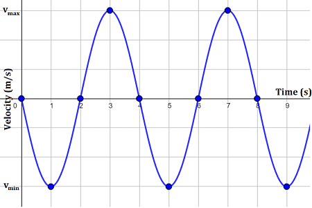
Graphical Analysis Techniques
Many AP Physics problems present graphical data that you must interpret:
Position vs. Time Graphs:
- Amplitude = maximum displacement from equilibrium
- Period = time for one complete cycle
- Phase can be determined from initial conditions
Energy vs. Position Graphs:
- Turning points occur where KE = 0 (total energy = potential energy)
- Equilibrium corresponds to minimum potential energy
- The shape of the PE curve determines the type of oscillation
Velocity vs. Position Graphs:
- These produce elliptical curves for SHM
- Maximum velocity occurs at equilibrium (x = 0)
- The area enclosed is proportional to the total energy

Connecting Oscillations to Waves
Unit 7 serves as a crucial bridge to understanding wave phenomena in later physics courses. The mathematical descriptions of oscillations directly extend to wave motion.
The Oscillation-Wave Connection
A wave can be thought of as oscillations that propagate through space. The equation for a traveling wave:
y(x,t) = A sin(kx – ωt + φ)
closely resembles our SHM position equation, with the addition of spatial dependence through the wave number k.
Standing Waves and Normal Modes
When waves reflect back and forth in a confined space, they can form standing wave patterns with specific frequencies called normal modes. These modes represent the natural oscillation frequencies of extended objects like guitar strings or organ pipes.
For a string of length L fixed at both ends:
fn = (n/2L)√(T/μ)
where T is the string tension and μ is the linear mass density.
Real-World Physics: Every musical instrument creates sound through oscillations at specific normal mode frequencies. When you press a fret on a guitar, you’re effectively changing the length L and thus shifting all the normal mode frequencies-this is how you change the pitch.
Common Misconceptions and How to Overcome Them
Through years of teaching AP Physics, certain misconceptions appear consistently among students. Recognizing and addressing these early will significantly improve your problem-solving success.
Misconception 1: “Heavier objects oscillate faster”
The Reality: For both pendulums and mass-spring systems, the period formulas show that mass either doesn’t affect the period (pendulum) or causes longer periods (mass-spring system). This counterintuitive result reflects the balance between inertial and gravitational effects.
How to Remember: Think of a grandfather clock-making the pendulum bob heavier doesn’t make it tick faster.
Misconception 2: “Larger amplitudes mean higher frequencies”
The Reality: For true simple harmonic motion, frequency is independent of amplitude. This is called isochronism and is what makes pendulum clocks accurate timekeepers.
How to Remember: A guitar string plays the same note whether you pluck it gently or vigorously-the loudness changes (amplitude) but not the pitch (frequency).
Misconception 3: “Energy is lost during oscillation”
The Reality: In ideal SHM, mechanical energy is perfectly conserved, continuously transforming between kinetic and potential forms. Energy is only lost in real systems due to friction, air resistance, or other dissipative forces.
How to Remember: Energy isn’t destroyed-it just changes forms. In a frictionless oscillator, the energy keeps bouncing back and forth between kinetic and potential, just like a perfectly elastic collision.
Misconception 4: “The restoring force is strongest at equilibrium”
The Reality: The restoring force is zero at equilibrium and strongest at maximum displacement. This is why objects momentarily stop at the turning points-the force is maximum there, but it takes time to accelerate the object back toward equilibrium.
How to Remember: Springs push back hardest when stretched the most, not when they’re at their natural length.
Laboratory Investigations and Data Analysis
The AP Physics 1 exam places significant emphasis on experimental design and data analysis skills. Unit 7 provides excellent opportunities to develop these competencies through hands-on investigations.
Investigation 1: Pendulum Period Relationships
Objective: Determine how pendulum period depends on length, mass, and amplitude.
Experimental Design:
- Variable Testing: Systematically vary one parameter while holding others constant
- Data Collection: Time multiple oscillations to reduce measurement uncertainty
- Graphical Analysis: Plot appropriate variables to linearize relationships
Expected Results:
- Period vs. Length: T ∝ √L (linear when plotting T² vs. L)
- Period vs. Mass: No dependence (horizontal line)
- Period vs. Amplitude: No dependence for small angles (horizontal line)
Common Experimental Errors:
- Large angle effects: Using amplitudes > 15° introduces nonlinearity
- Timing consistency: Starting and stopping the timer at the same point in the cycle
- Length measurement: Measuring to the center of mass of the bob, not the bottom
Investigation 2: Mass-Spring System Analysis
Objective: Verify the relationship T = 2π√(m/k) and explore energy transformations.
Advanced Techniques:
- Video analysis: Use slow-motion video to track position vs. time
- Force sensors: Directly measure the restoring force at different displacements
- Energy calculations: Calculate kinetic and potential energy at various points
Data Analysis Skills:
- Linearization: Transform nonlinear relationships into linear forms for easier analysis
- Error propagation: Understand how measurement uncertainties affect calculated results
- Model validation: Compare experimental results to theoretical predictions

Practice Problems: Mastering the AP Format
The following problems represent the variety and depth you’ll encounter on the AP Physics 1 exam. Work through them systematically, focusing on both mathematical solutions and conceptual understanding.
Problem 1: Multiple Choice (Energy Analysis)
A mass oscillates on a spring with amplitude A and period T. At what displacement from equilibrium is the kinetic energy equal to the potential energy?
(A) A/4
(B) A/2
(C) A/√2
(D) 3A/4
(E) A
Solution: At any point in SHM, total energy E = KE + PE. When KE = PE, we have:
KE = PE = E/2
Since E = ½kA² and PE = ½kx², we get:
½kx² = ¼kA²
x² = A²/2
x = A/√2
Answer: (C)
Conceptual Understanding: This occurs at the point where the object has converted exactly half its total energy to each form-a natural consequence of the quadratic relationships in harmonic motion.
Problem 2: Free Response (Experimental Design)
A student wants to determine the spring constant of an unknown spring using a set of masses and a timer.
(a) Describe an experimental procedure to determine the spring constant, including what measurements to take and how to analyze the data.
(b) Identify two sources of systematic error that could affect the results and explain how each would impact the calculated spring constant.
(c) The student obtains the following data:
| Mass (kg) | Period (s) |
|---|---|
| 0.10 | 0.89 |
| 0.20 | 1.26 |
| 0.30 | 1.54 |
| 0.40 | 1.78 |
| 0.50 | 1.99 |
Determine the spring constant from this data and estimate the uncertainty in your result.
Solution:
(a) Experimental Procedure:
- Attach different masses to the spring and allow each to reach equilibrium
- Displace each mass slightly and release, timing 10 complete oscillations
- Calculate period T for each mass: T = (total time)/10
- Plot T² vs. m (should be linear based on T = 2π√(m/k))
- Calculate spring constant from slope: slope = 4π²/k
(b) Sources of Systematic Error:
- Air resistance: Would increase the period slightly, leading to an underestimate of k
- Mass of spring: The spring’s own mass effectively adds to the oscillating mass, also leading to an underestimate of k
(c) Data Analysis:
Creating a table of T² vs. m:
| Mass (kg) | T² (s²) |
|---|---|
| 0.10 | 0.79 |
| 0.20 | 1.59 |
| 0.30 | 2.37 |
| 0.40 | 3.17 |
| 0.50 | 3.96 |
The linear relationship gives: slope = 7.9 s²/kg
Therefore: k = 4π²/slope = 4π²/7.9 = 5.0 N/m
Problem 3: Conceptual Reasoning (Pendulum Analysis)
Two identical pendulums are set up, one on Earth and one on the Moon (where g = 1.6 m/s²). Both pendulums have the same length and are released from the same angle.
(a) Compare the periods of the two pendulums. Justify your answer.
(b) Compare the maximum speeds of the pendulum bobs. Justify your answer.
(c) If both pendulums start with the same total energy (as measured in their respective reference frames), compare their amplitudes. Explain your reasoning.
Solution:
(a) Period Comparison:
Since T = 2π√(L/g), and gMoon = gEarth/6.25:
TMoon = 2π√(L/1.6) = 2.5 × 2π√(L/9.8) = 2.5 × TEarth
The Moon pendulum has a period 2.5 times longer.
(b) Maximum Speed Comparison:
Maximum speed occurs at equilibrium: vmax = Aω = A√(g/L)
Since gMoon < gEarth, the Moon pendulum has a smaller maximum speed for the same amplitude.
(c) Amplitude Comparison:
For the same total energy E = ½mgLA²/L = ½mgA² (small angle approximation):
If EMoon = EEarth, then:
½mMoonAMoon² = ½mEarthAEarth²
Since gMoon < gEarth, AMoon > AEarth to maintain the same energy.
Conceptual Understanding: Gravity affects both the restoring force and the potential energy reference, leading to these interconnected relationships.
Advanced Topics: Beyond the AP Curriculum
While not required for the AP exam, understanding these advanced concepts will deepen your appreciation for oscillatory phenomena and prepare you for future physics courses.
Coupled Oscillators
When two or more oscillators interact, they can exchange energy in fascinating ways. Consider two identical pendulums connected by a weak spring. If you start one pendulum swinging while the other is at rest, you’ll observe the energy gradually transfer from the first to the second, then back again—a phenomenon called beating.
Nonlinear Oscillations
Real oscillators often deviate from simple harmonic motion when amplitudes become large. For a pendulum, the small angle approximation breaks down, and the period begins to depend on amplitude. The exact formula for a pendulum’s period involves elliptic integrals-advanced mathematical functions that account for these nonlinear effects.
Quantum Harmonic Oscillator
At the atomic scale, oscillations take on quantum properties. The quantum harmonic oscillator serves as the foundation for understanding molecular vibrations, phonons in solids, and even the vacuum fluctuations of electromagnetic fields. The energy levels become quantized: E = ℏω(n + ½), where n is an integer and ℏ is Planck’s constant.
Technology Applications: Oscillations in the Digital Age
Modern technology relies heavily on oscillatory phenomena, often in ways that aren’t immediately obvious.
Quartz Clocks and Watches
The incredible accuracy of quartz timepieces stems from the piezoelectric properties of quartz crystals. When subjected to an electric field, quartz crystals oscillate at extremely stable frequencies—typically 32,768 Hz for watch crystals. This frequency is chosen because it’s a power of 2 (2¹⁵), making it easy to divide down to 1 Hz using digital circuits.
Atomic Clocks
The world’s most precise clocks use the oscillations of atoms themselves as timekeeping references. Cesium atomic clocks define the international standard for time, based on the frequency of electromagnetic radiation emitted when cesium atoms transition between specific energy levels.
Touch Screens and Sensors
Capacitive touch screens work by detecting changes in oscillating electric fields when your finger approaches the surface. Your finger effectively becomes part of an oscillating circuit, changing its natural frequency in a way that electronics can detect and locate.
Seismic Monitoring
Networks of sensitive oscillators (seismometers) continuously monitor Earth’s vibrations, detecting everything from distant earthquakes to underground nuclear tests. The analysis of seismic oscillations has revealed the internal structure of our planet and provides early warning for tsunamis.

Study Strategies for AP Success
Mastering Unit 7 requires both conceptual understanding and mathematical fluency. Here’s a comprehensive approach to maximize your preparation:
Foundation Building
- Master the basic definitions: period, frequency, amplitude, phase
- Understand the force-motion relationship: F = -kx and its implications
- Practice energy analysis: KE ↔ PE transformations
- Work through derivations: Don’t just memorize formulas-understand where they come from
Problem-Solving Flowchart
When approaching any oscillation problem:
- Identify the system type (pendulum, mass-spring, etc.)
- Find the equilibrium position (where net force = 0)
- Choose your approach:
Formula Summary and Quick Reference
Essential Relationships:
- Simple Harmonic Motion: x(t) = A cos(ωt + φ)
- Angular frequency: ω = 2πf = 2π/T
- Mass-spring system: T = 2π√(m/k)
- Simple pendulum: T = 2π√(L/g)
- Energy relationships: E = ½kA² = ½mω²A²
Conclusion: The Rhythm of Physics
As you complete your journey through AP Physics 1 Unit 7, you’ve gained insight into one of nature’s most fundamental patterns. From the atomic vibrations that determine material properties to the oscillations of space-time itself in gravitational waves, the principles you’ve learned govern phenomena across an incredible range of scales.
The mathematical elegance of simple harmonic motion-with its perfect balance of forces, smooth energy transformations, and predictable periodicity-represents physics at its most beautiful. Yet this beauty isn’t merely aesthetic; it’s practical. Engineers use these principles to design earthquake-resistant buildings, musicians rely on them to create pleasing sounds, and scientists apply them to probe the deepest mysteries of the universe.
Your success on the AP exam will depend not just on memorizing formulas, but on developing a deep intuitive understanding of how oscillatory systems behave. When you can visualize the interplay between restoring forces and inertia, when you can predict how changing parameters affects motion, and when you can design experiments to test your predictions-that’s when you’ve truly mastered oscillations.
Remember that physics is ultimately about patterns and connections. The oscillation concepts you’ve learned will appear again in waves, electricity and magnetism, and quantum mechanics. Each new context will deepen your understanding and reveal new applications of these fundamental principles.
As you prepare for the AP exam, focus on understanding rather than memorization. Work through problems systematically, always asking yourself “Why?” and “What if?” Connect the mathematics to physical reality, and don’t be afraid to use your intuition-properly trained physical intuition is one of the most powerful tools a physicist can possess.
The rhythm of oscillations surrounds us constantly, from the beating of our hearts to the vibrations of our smartphones to the oscillations of electromagnetic fields that bring us light and radio waves. By understanding these patterns, you’ve gained insight into the fundamental mechanisms that make our world work.
Now go forth and oscillate-with confidence, understanding, and the solid foundation that will serve you well in whatever scientific endeavors await you!
Recommended –
2 thoughts on “Mastering AP Physics 1 Unit 7: Oscillations – The Complete Guide to Periodic Motion”